Now that we’ve gotten rid of all the estimators we don’t want (i.e. those that aren’t RAL), we need to figure out how to sort through the all remaining estimators we might have at our disposal:
So let's do just that. By imposing asymptotic linearity, we've actually made our job super easy. As gets bigger and bigger, we know that the sampling distribution of any RAL estimator minus truth (scaled by root ) goes to a normal with mean zero and variance given by where is the influence function for that particular estimator. That means that the only difference between any two RAL estimators (in large enough samples) is that they have sampling variances of different magnitude. Obviously we would prefer an estimator with less variance because that will give us smaller (but still valid) confidence intervals and p-values. In other words, given the same data, we are more certain of our estimate if we use an estimator that has a smaller sampling variance.
The implication is that, if given the choice, we want to pick an estimator with an influence function that has the smallest possible variance.
However, instead of picking an estimator out of a lineup, why don't we make our own estimator that is guaranteed to beat anything that anyone else could come up with? Here is a strategy that will let us do that:
Figure out the set of all possible influence functions:
Pick the one that has the smallest variance:
Build an estimator that has that influence function.
This section will cover steps 1 and 2 of this strategy. There are a few different strategies to build an estimator that has the influence function with smallest variance and these will be the subject of the next chapter.
It's important to come away with an understanding of what and the why of what we're going to discuss. In practice, unless you're working with brand-new model spaces or parameters, you will never have to actually do any of what is described in this section. Nonetheless it's critical to understand it to have an idea of how the tools we have today were developed and why they work.
Characterizing the Set of Influence Functions
Not every possible function corresponds to a valid RAL estimator in a particular statistical model. For example, it would be great if we could find a RAL estimator with because this estimator would have no variance at all in large samples. Clearly that's a pipe dream that's not going to happen in general, so we must conclude that is not an influence function. For a given parameter and statistical model, what functions are influence functions of RAL estimators, and what functions aren't?
Using nothing but the definitions of regularity and asymptotic linearity, we arrive at the following result. For any RAL estimator with influence function , the following holds for all scores corresponding to paths in the model:
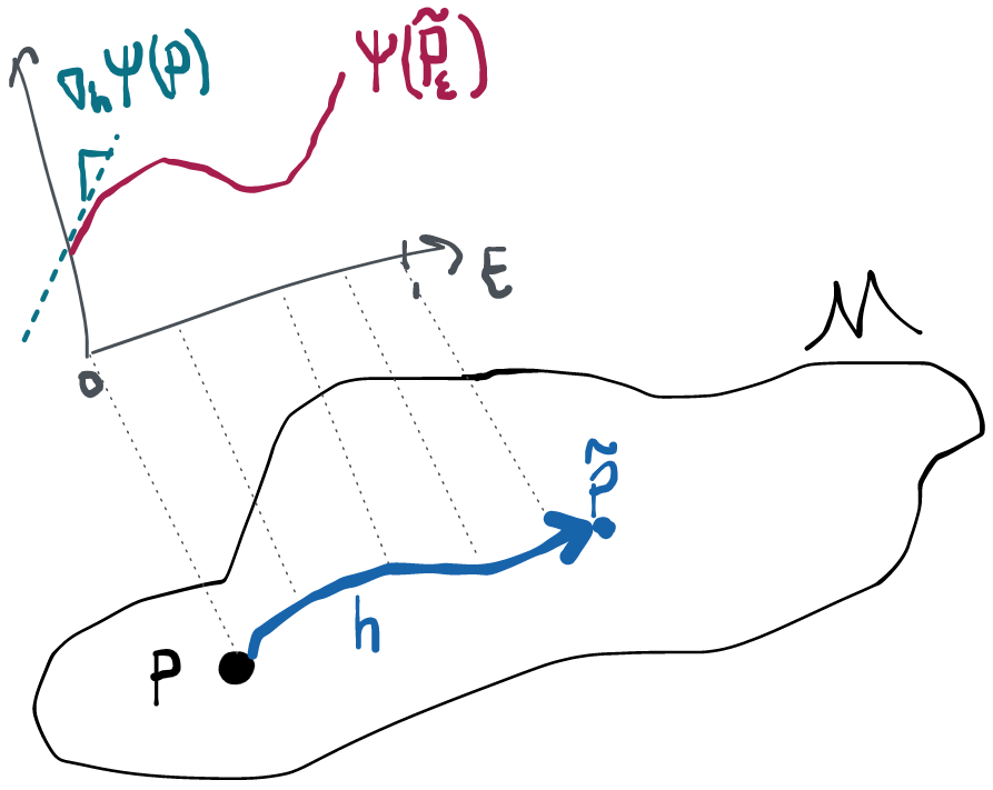
Before giving a proof, which sadly relies on some technical results, let's understand what this is even saying. The term on the left is what we call the pathwise derivative of at in the direction (evaluated at 0). From now on we'll abbreviate this with the notation . The term on the right is the covariance between and because both are mean-zero. So what the result above says is that
[Reisz representation, central identity for influence functions] If is an influence function for a RAL estimator of a parameter and is the score for any legal path at , the -direction pathwise derivative of is equal to the covariance of and :
This is a fascinating connection between what seem to be two very different things. The pathwise derivative describes how quickly the estimand (parameter) changes as we move along a particular path. The expectation of the influence function times the score effectively tells us what the angle is between the path's score and the estimator's influence function (see section below on the space if this confuses you). The left-hand side (pathwise derivative) depends on the parameter , the direction , and the true distribution . The right hand side (influence function covariance w/ score) depends on the choice of estimator, implying , the direction , and the true distribution (under which the covariance is taken).
This is cool in and of itself, but it's also the fundamental key to characterizing the set of all influence functions, and therefore the key link that holds everything we're talking about together.
😱 Proof that
We'll start with our definition of a path and our definition of asymptotic normality. Using just these definitions and some esoteric theorems, we'll amazingly be able to characterize how our estimator should behave as we move along the path towards . That's a little surprising because asymptotic normality is a property that only holds at and doesn't say anything explicit about behavior along paths. Nonetheless, we'll see that there is an implication for how the estimator behaves along paths. However, we've also assumed the estimator is also regular, which is already a definition of how the estimator behaves along paths. In comparing the derived behavior from asymptotic normality and the assumed behavior from regularity, we will see there is a difference. The difference in the two behaviors can only be made to go away (as it must if an estimator is both asymptotically normal and regular) if , so that's what we conclude.
In proving that asymptotic normality and our definition of a path by themselves imply some behavior of the estimator along such a path we'll have to use two advanced, technical results. Unfortunately I haven't found an alternative way to prove this that is both rigorous and intuitive. It's not at all impossible to understand these theorems (just read the appropriate sections of vdW 1998) but if you're not interested in the math for its own sake it's probably not worth your time. In terms of understanding the arc of the proof you just need to grasp how we've used these tools to get what we need, not how they work.
Throughout I'll abbreviate (the estimate as we draw increasing samples from ) and (the true parameter at ) to keep the notation light. I'll also abbreviate , which is the estimate as we draw increasing samples from distributions moving along our path closer to , and , which are the true parameter values at each of these distributions. Anything that has a hat is an estimate, anything that has a tilde is along a path.
Alright, go time. Let's see what we can say about how our estimator behaves along sequences of distributions like , since these are the only ones regularity has anything to say about. By theorem 7.2 of vdV 1998 the fact that our paths are differentiable in quadratic mean ensures that we get something called local asymptotic normality 🤷:
It really doesn't matter what this means because we're just going to use it to satisfy a particular technical condition in a minute. The important part is to see that we've defined some random variable on the left: the derivative-looking thing is just some fixed function of the data, so let's rename that as some random variable . What the right hand says is that in large-enough samples, this thing looks like a sum of IID variables plus some constant. We combine this with the assumed asymptotic linearity of our estimator:
Which is also a random variable that's approximately equal to an IID sum when gets big. Here we stack the two above equations on top of each other and by the central limit theorem we have that
Now we use another technical result 🧐 (Le Cam's 3rd lemma- see vdV 1998 ex. 6.7), which says that when we have exactly the situation above, we can infer
Again it's not important to understand the technical device. The idea is that we're trying to say something about how our estimator behaves as we change the distribution along our path of interest. At first this seems impossible because asymptotic normality only holds at each and doesn't say anything about what happens along paths. However, with the help of these technical devices, we've actually managed to say something about the difference between the estimate as we change the underlying distribution and the truth at . In particular, this difference converges to a normal with the same variance as if we had not been moving along the path towards but had instead sat still at . Crazy. The limiting normal distribution now has some mean , which we'll pull out in the course of some algebraic manipulation during which we also add and subtract on the left:
Moving terms around, we arrive at
Notice that the term in brackets on the left is a constant for each , i.e. it's not random.
Now, finally, we recall our definition of regularity, which was
An estimator that is asymptotically linear must satisfy the behavior in the display above denoted (AL). An estimator that is regular must satisfy the behavior in the display denoted (R). A RAL estimator must satisfy both. But the only way that both of those can be true is if they are actually saying the same thing, which only happens if the bracketed term in (AL) goes to zero. Thus, for RAL estimators,
where we've recalled from our original definition of our sequence along the path.
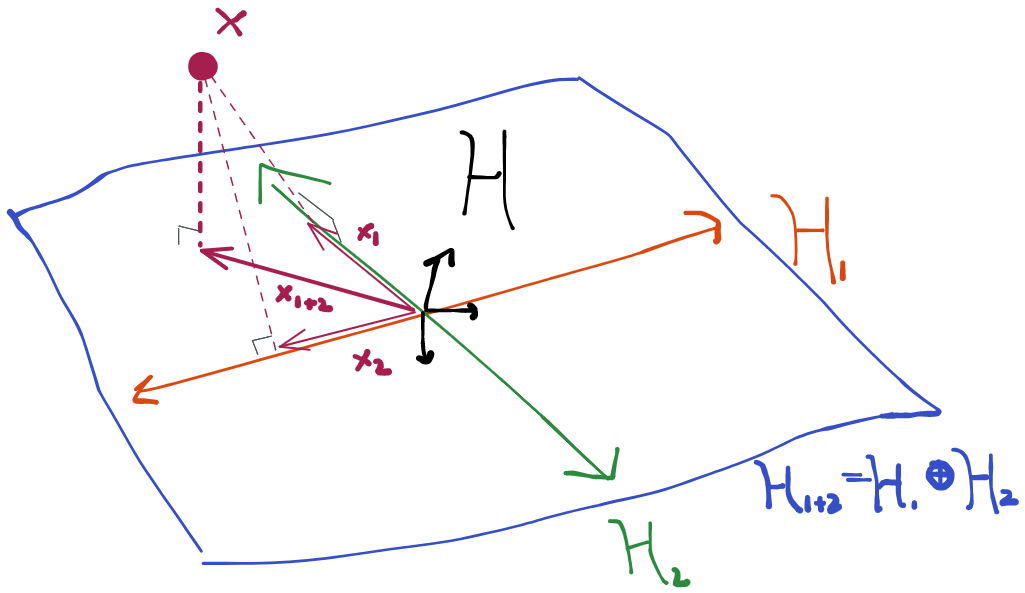
What we mean is this: since the left-hand side doesn't depend on the influence function , the same identity holds (keeping constant and ) for any two estimators with influence functions , (if two such estimators exist). Specifically: . Eliminating the middleman, we get . Therefore the difference of influence functions for any two RAL estimators is orthogonal to any score! If you don't understand why this is the implication, you should review the section on space. Moreover, if we take any function that is orthogonal to all scores and add it to the influence function from a RAL estimator, the result still satisfies the above requirement and so this is an influence function for a different RAL estimator.
The Space
We can treat any score and any influence function as an element of a set we call (or just when the measure is clear). This is the set of all functions which satisfy the condition (i.e. is a random variable with finite variance). This space is a lot like the vector space in many important ways:
is a linear space:
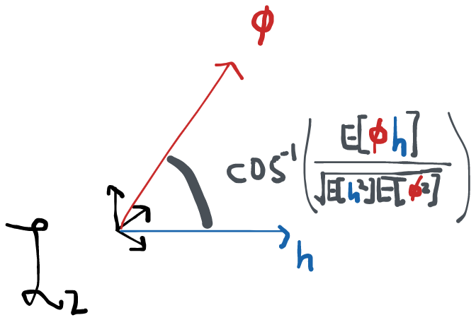
has an inner product: in , the inner product between two vectors and is given by . The equivalent in for two functions and is . Note how the integral of a product of two functions is a lot like the sum of the element-wise product of vectors. It happens that the two operations obey all the same rules that define something as an "inner product". When we don't have a specific space in mind, we usually write the inner product between two elements as . If two elements have an inner product equal to 0 we say that the two are orthogonal. This generalizes the notion of two vectors being at a right angle in . More generally, the inner product also defines what the "angle" is between two vectors: , where is the norm of in this space.
is complete. This is a technical term that means that the space contains all of its limit points (i.e. a sequence of convergent elements in the space can't converge to a limit that is outside the space).
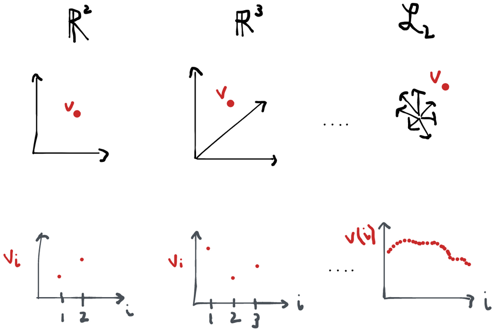
Together, these conditions are the definition of something called a Hilbert space. Indeed, and are the usual examples of Hilbert spaces. The main difference between the two is that is finite-dimensional, whereas is infinite-dimensional. What do I mean by this? Well, a vector in, say clearly has 3 components . A "vector" in has as many components as its functions have arguments because you can think of a function like this: . The only difference is that I put the "vector index" in parentheses instead of as a subscript and now I call it an "argument". We also now allow for indices that are anywhere in the domain of instead of just the integers . Alternatively, we can think of the vector as a function that maps . So vectors, functions, whatever. It's kind of the same thing in most of the ways that matter!
Tangent Spaces
If influence functions are orthogonal to every score , they must also be orthogonal to any linear combination of scores, or any limit of a sequence thereof. So it makes everything more concise if we start talking about the tangent space (which is exactly the set of all scores, their linear combinations, and limits) instead of having to continually refer to "all scores". Since the tangent space comes from the set of scores, it has nothing to do with either the estimator or the parameter. It depends purely on the statistical model and the true distribution .
Why is it called the tangent space?
Honestly, I don't think it's the greatest name, but let's explain it.
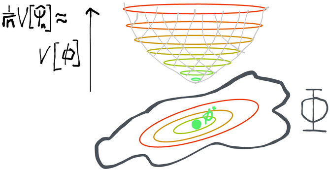
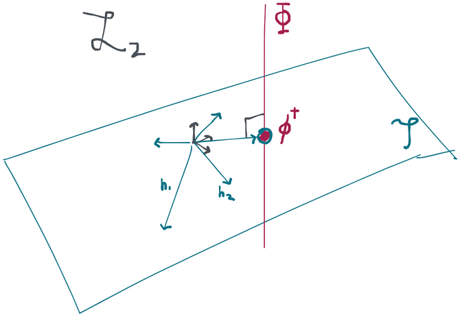
The key is to 1) think about each point as having density w.r.t. some dominating measure and 2) realize that . Because has to integrate to 1, then then norm of (that is, is of course 1. So we can identify with some subset of the unit ball in . It's now easy to show that is orthogonal to :
so the set of functions ranging over scores is orthogonal (tangent) to the point in the model space. Or, equivalently, is orthogonal to all scores in the space .
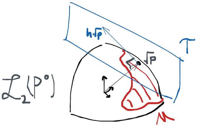
Once nice thing that this picture shows is that the tangent space clearly depends on where is within the model.
Nonetheless, it'd probably be more informative to call it the "score space", since the fact that the scores are tangent to the density in doesn't seem matter that much in terms of the role the space ends up playing in the theory we're developing. Alas, we're stuck with the names we have.
Saturated vs. Non-Saturated Models
Sometimes the tangent space is all of . This happens if we put no restrictions on the distributions in our statistical model. If any distribution can be in the model, then starting at any point , any function that has zero mean and finite variance defines a valid path at because will still be a density for any such score .
When this happens, we say that the model is nonparametric saturated, or just saturated (at ). Intuitively, this means that we have a model space such that, standing at , we can move in any direction and still stay inside the model. If this is not the case, then we say the model is not saturated (at ).
Factorizing Tangent Spaces
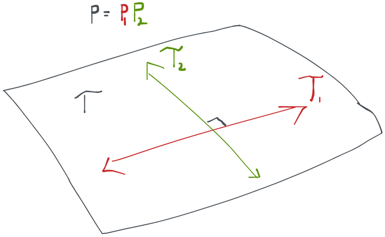
While we're on the subject of tangent spaces, it turns out that if we can factorize our distribution then all scores end up being the sum of scores for each factor, treating these as living in statistical models of their own, i.e. . Moreover, the scores for each factor end up being orthogonal, i.e. and . Lastly, these scores satisfy and . A short proof of all of is given below. This argument also generalizes to densities that have more than two factors (just factor one of the two factors).
Proof
Recall that . For small enough is still in the model, so we can factor it into (omitting the subscripts). The log of a product is the sum of logs and the derivative is linear over a sum, so we get
Now we'd like to show that in .
For that we have to notice that is a score at in the nonparametric model (by definition). If we start at and move along a path defined by , the only way we stay within is if . Otherwise the resulting perturbation will not be a density. Similarly, we need for .
Now and we've shown and are orthogonal.
We can also go the other way- if I propose and that satisfy the above, then must be a valid score at in the original model.
Variational Independence
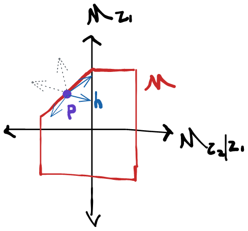
We showed that the tangent space can be broken up into an orthogonal sum when every distribution in the model factors and those factors can vary independently in their own model spaces. There are cases where this breaks down, though. If you look at the following picture, you'll surmise that all the scores at (blue arrows) can indeed be created as orthogonal sums of scores from and . However, there are arrows that can be constructed the same way (grey, dotted) that take us outside of the model space- these are not scores because they don't correspond to a legal path inside the model. Therefore in this case , but we don't have the equality. When this happens, we say that our submodels are not variationally independent. In other words, there are some points in the model space where I can't legally change in one of the submodels without having to make a change in another (i.e. at in the picture we can't go just up, we also have to move a bit to the right along the diagonal).
We can therefore usually construct tangent spaces for each factor separately and then the tangent space for the whole model is the orthogonal sum of the component tangent spaces (we write this ).
Consider what happens if we perturb a density along a path defined by a score that satisfies and . We know that , but what can we say about the resulting factors and ? A bit of algebra using the properties of and the definition of the conditional density shows that and also . In other words, moving along a path in only affects the factor . Similarly, if you repeat this exercise with a score satisfying you get that and also . Thus moving along a path in only affects the factor . This should make some intuitive sense to you, and, naturally, everything generalizes cleanly when there are more than two factors.
This is useful when we evaluate the directional derivative . If is the sum of two other functions we can always write because the derivative is a linear operator in the score. The resulting terms and are now easier to evaluate because for each of them we just need to consider a single perturbation in or in , respectively. We’ll see this come in handy in the next section of this chapter.
Example: tangent space for a randomized controlled trial
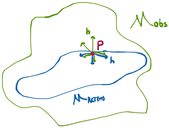
Let's give a concrete example of a tangent space at for some particular statistical model. For our model, we'll use the space where RCT() stands for "randomized controlled trial" with treatment mechanism . This model is characterized by a joint distribution between some vector of observed covariates , a binary treatment , and an outcome . Any distribution of three variables can always factor as . The treatment mechanism is defined as , the probability of receiving treatment given observed covariates .
What makes the RCT model space different from the more general nonparametric space where each of these three distributions can be anything is that in the RCT the distribution of is fixed. Specifically, we know . For example, in a trial with a simple 50:50 randomization we have .
So what are the possible scores? The density factors into three components, only two of which can actually vary. Thus any score will be the sum of two orthogonal components, one of which corresponds to and one of which corresponds to (recall is fixed so we can't move in that "direction").
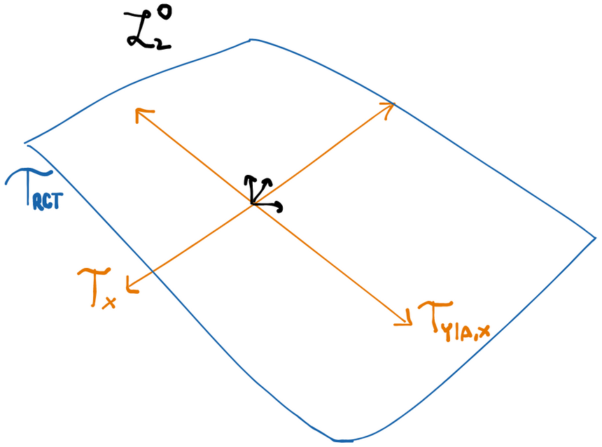
Now we're basically done. Since there are no more restrictions on our model, our tangent space is orthogonal sum of the two tangent subspaces. Let be the subspace of all zero-mean functions in (recall all scores and all influence functions have mean zero). Now, formally:
Can you think of a function that is in but not in ?
Example: tangent space for an observational study
The difference between the observational study model and the RCT model is that now we don't know the treatment mechanism . This model (we'll call it ) therefore contains for any treatment mechanism .
Since this model is larger than , it should make some intuitive sense to you that the tangent space is bigger too. This is because at any point in the model, we have more directions we can move in than we previously did. Specifically, we can now move in directions that end up changing the treatment mechanism. To be specific, we can have paths through (specified by some ) such that . But this same cannot be a path through because for the fluctuated distribution to remain inside of we have to require that . Therefore for any with some treatment mechanism , all paths through in are also paths through in but not vice-versa.
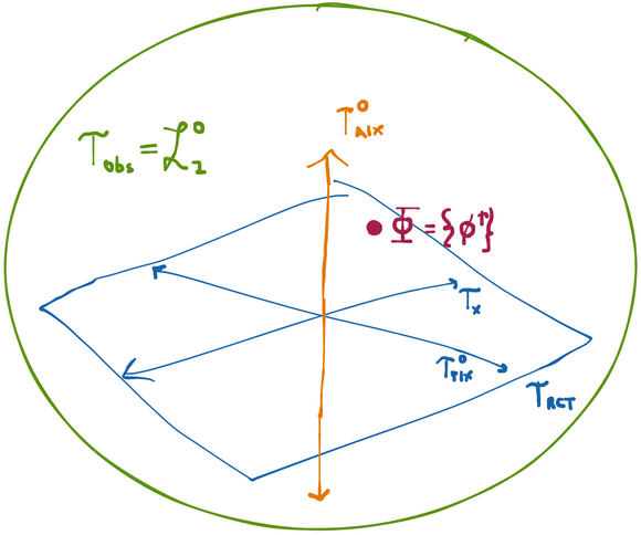
We can be even more specific about this. Since any density in factors as we immediately have that the tangent space is given by the orthogonal sum . Compare this to and you immediately see that scores in the observational study have an additional set of degrees of freedom that the score in the RCT don't have. Namely: all directions in . In fact, , which is to say that any mean-zero function with finite variance is a legal score for this model. That's because we've put literally no restrictions on what can be so is a legitimate density in our model for any such .
The Efficient Influence Function
Starting with nothing but the definition of a RAL estimator, we've shown that the set of influence functions of RAL estimators is (after shifting it to the origin) orthogonal to the tangent space. Since RAL estimators basically only differ by their variance (which is the variance of their influence functions), we get the best RAL estimator by finding one that has the influence function with the smallest variance. The point of everything we've done in the section above is that at least now we know the space we have to look in!
Thankfully, our characterization of the tangent space and the set of influence functions makes it easy to find the influence function with the smallest variance.
Pathwise Differentiability
There are combinations of parameters and models for which the pathwise derivative doesn't exist or isn't a bounded linear operator. For example, consider densities of and let our parameter be for a particular point of interest . You can evaluate the derivative and show that . The problem here is that I can always pick with norm 1 but that takes huge values at (by compensating with large negative values at other ). So I can pick (in the unit ball) such that the integral blows up as large as I want. That's what "unbounded" means for a linear operator. The consequence of this is that the Reisz representation theorem no longer applies and we cannot guarantee that there is an element that is in the tangent space. This also destroys the argument based on the difference of two influence functions of RAL estimators because we can't guarantee that even a single RAL estimator exists.
To do this we can argue that there is some influence function that is itself in the tangent space because we can always project some influence function into to get . By definition, is in the tangent space, and by what we know about the relationship of to the tangent space, is the difference of an influence function with something that's orthogonal to all scores, meaning that it too must be an influence function. We can reach the same conclusion if we use the Reisz representation theorem. If the pathwise derivative, viewed as a function of the score , is bounded and linear among scores in , then there is some element of that satisfies our requirement of being an influence function for a RAL estimator. This is is usually the case, although there are some parameters and models for which it isn't. But as long as we have pathwise differentiability, there is always exactly one influence function that is also in the tangent space.
Reisz Representation
Besides giving us a definition of orthogonality, Hilbert spaces are super nice to work in because of an important property called Reisz representability. The Reisz representation theorem says that if you have a bounded linear function that maps an element of the Hilbert space to a real number, then that function can always be represented as an inner product between the argument to the function and some other element of the Hilbert space. In other words, for every bounded linear function , there is some element so that .
This is a very surprising result at first but it's pretty easy to convince yourself of it in . Consider vectors (I'll use the vector arrow in this section to be very explicit). The definition of a linear function is that for any scalar . Any linear function in this particular space is bounded so we don't need to worry about what that means. To show that is actually just taking an inner product between and some other vector we can apply to the unit vectors and see what it returns. Say . Now we can express any vector as the weighted sum of the unit vectors , and by linearity of notice now that . The conclusion is that the operation of the function on is really just the inner product between and some other vector , which is also in . The other direction is also obvious: given , define and since the inner product is a linear operation in both arguments, we have that the function is linear as desired.
What's amazing is that this property actually extends to any Hilbert space (i.e. a complete linear space with an inner product). In particular, if we have a bounded linear function that maps functions to real numbers, then we know there is some fixed function such that . If you're unfamiliar with functions that have functions as arguments you can think of as "assigning" a number to each function .
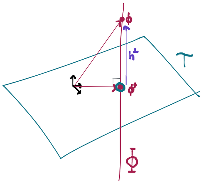
Projection in Hilbert Space
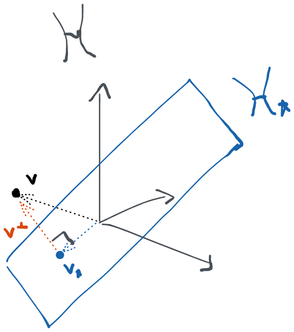
Almost all Hilbert spaces contain other Hilbert spaces within them. For example, we can think of any plane in 3D space as a 2D space in its own right. If we add the restriction that the contained space must have the origin in it, we call it a subspace and a useful result follows. Namely: for every vector in the Hilbert space , there is always exactly one vector in the desired subspace and a vector that's orthogonal to every vector in such that . Since the projection is unique, it's easy to check if is indeed a projection by simply checking (1) whether and (2) whether .
If a subspace is the orthogonal sum of two other subspaces, we can always obtain the projection by projecting into each sub-subspace and then summing the result.
And, in fact, this unique influence function in the tangent space is the one with the smallest variance. The proof of this is relatively simple: and are subsets of . In this space, the norm is since by definition must have mean zero to be in . Therefore looking for the smallest variance influence function is the same as looking for the influence function with the smallest norm in , or, equivalently, the point in that's closest to the origin. We can write any point in as the sum of the influence function that is in the tangent space plus some function that is orthogonal to the tangent set: . But since those two components are at a right angle, there's no way for the length of the "vector" to be less than the length of the "vector" because the Pythagorean theorem says that .
Because has the smallest variance of any influence function, and therefore any RAL estimator that has it will make the most efficient possible use of the data, we call the efficient influence function (EIF; sometimes also referred to as efficient influence curve or EIC).
If we identify as the unique element in the tangent space for which the pathwise derivative in a particular direction can be represented as the inner product between that direction and this element (i.e. the Reisz representation), then it also makes sense to call the canonical gradient.
Why is it called the canonical gradient?
If we have a function that maps vectors to real numbers, the directional derivative at in the direction of a vector is defined as . However, it's well-known that we can also write this as the sum of the partial derivatives times the components of : . In fact, the proof of this follows from noticing that the directional derivative is a linear operator and applying the Reisz representation theorem that we derived for finite dimensional . Of course, this is the same as the inner product between the vector of partial derivatives, which we call the gradient , and . Thus .
Now it should make sense why we refer to as a gradient. It's exactly the same as , except now we're in instead of . Since we can write the directional derivative as an inner product , the object is serving exactly the same role as the gradient is above. To reiterate:
We call the canonical gradient because there are usually many functions in that satisfy the above (namely: every other influence function). However, is the only one that is in the tangent space, and is the only one that's guaranteed to exist according to the Reisz representation theorem. That's what makes it "canonical".
In the context we've described here it might make more intuitive sense to use the notation to represent the canonical gradient. However, we use to make the connection to influence functions for RAL estimators. A gradient (depends on the parameter) and an influence function (depends on the estimator) are actually totally different things. It just so happens that for RAL estimators they happen to occupy exactly the same space.
If a model is saturated, these geometrical arguments imply that there is only one valid influence function (and it is therefore efficient). To see why, we'll assume that there are two different influence functions and then show that they are actually the same. If there are two IFs, we know that for all in the tangent set, which in the case of a saturated model is all of . However, is itself a zero-mean, finite variance function (i.e. an element of the tangent set) so there is some score . But by the orthogonality result, we must have that . Since nothing can be orthogonal to itself unless it is 0, we conclude that and our two "different" influence functions are in fact the same one. This, in turn, means there exists only one RAL estimator (or, technically, one class of RAL estimators that are all asymptotically equivalent).