There are two kinds of conditions we want to satisfy before we'll consider an estimator "legitimate":
Is it practical to use? In other words, can we at a minimum assume that the estimator gets better in larger samples and that we have a good way to calculate confidence intervals? We'll call this property asymptotic linearity.
Is it robust? In other words, would this estimator still work if we slightly changed the true data-generating distribution? We'll call this property regularity.
Ultimately we will require that our estimator meet both these criteria to be considered. We'll call our final class of legitimate estimators regular and asymptotically linear (RAL). Before we get into these things, it's worth saying that practically all sensible estimators that you encounter in practice are RAL. So you shouldn't feel like we're making some arbitrary restrictions here that outlaw a bunch of popular estimators. We will now rigorously define what it means to be RAL.
Asymptotic Linearity
We want to be a "good" estimate of the estimand in some sense. But depends on the data, which is random, and so it is of course also a random quantity. Thus it's not sensible to desire something like "my estimate should always be correct" (i.e. ) because the estimand is a fixed number but the estimate will generally vary. A more sensible request might be "I want estimators that are correct on average", i.e. . However, it turns out that even this is usually a bit ambitious. In many problems there are no estimators that are always unbiased. Moreover, some estimators may very well have complicated, intractable sampling distributions that make it impossible to construct general-purpose confidence intervals or calculate p-values.
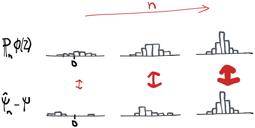
To resolve this, we can restrict our class of allowable estimators so that in large-enough samples they all have an approximately normal sampling distribution that converges to the true parameter value. The most convenient and general-purpose way to guarantee this is to restrict ourselves to estimators that are asymptotically linear. The definition of an asymptotically linear estimator is one that satisfies the following equation:
For some function such that .
Example: Asymptotically Linear Estimator
Consider the statistical model defined by all possible distributions of a univariate random variable and define our target parameter (the population mean).
Let our estimator be (i.e. the sample mean). Subtracting from both sides and multiplying by gives which shows that the influence function for this estimator in this model is .
Note that, 1) as is required, this function is zero-mean and 2) we can see that depends on what is because may be different for different .
Simply put, as gets big, the difference between our estimate and the truth behaves as if it were an average of IID variables (remember the notation is just a sample average- the "population" mean under the empirical measure ). Exactly what those IID variables are is determined by some zero-mean function (of the observed data ) which we call the influence function of the estimator. By definition, all asymptotically linear estimators have an influence function, and any estimator that has an influence function is asymptotically linear.
It's not immediately clear why "influence function" is an appropriate name for this function. It might be more appropriate at this point to call it the "linearizing transformation" of the data relative to the estimator or something like that, since it allows us to represent our estimator as a sum of IID terms in large samples. We'll see later why it's called the influence function.
You may also wonder about the in front. That serves to "blow up" the difference between the estimation error and the sample average, so what we're saying is that what remains actually goes to 0 faster than blows up (if it didn't, then the whole thing wouldn't converge). Why ? Because the central limit theorem says that is what converges to a stable normal distribution. Without the root , shrinks down to a thinner and thinner normal distribution until by itself it's just a spike at zero. So is what we need to multiply everything by so that we're saying that the difference of two stable normal distributions is zero.
Central Limit Theorem
The central limit theorem is a fundamental result of probability theory that says that the sampling distribution of the average of IID random variables (scaled by ) looks more and more like a normal distribution with mean and variance . Formally, .
The is necessary because otherwise the distribution gets infinitely narrow (centered on ) as increases. It happens that is exactly the amount you need to counteract the shrinkage and "stabilize" the variance.
The influence function generally depen{ds on the true distribution . In the example we gave above for the population mean, we found , which clearly depends on because the true mean can change as we vary the true distribution . Being asymptotically linear just means that for each there is some function such that the above holds. So it's more explicit to write but we'll omit the subscript unless it's necessary. This will become important later so make a mental note of it.
It's totally possible for two different estimators to have the same influence function. This is because two different algorithms can turn out to behave very similarly as the sample size increases. We'll also see this later when we discuss different strategies for building optimal estimators: the estimators we get from using each strategy may be different, but they all have the same influence function and therefore all behave identically in large-enough samples.
Using the definition of asymptotic linearity it follows immediately from the central limit theorem that . In other words, by imposing asymptotic linearity, we ensure that the sampling distribution of our estimator is normal with mean zero as the sample size increases. That guarantees that our estimator is asymptotically unbiased (i.e. gets the right answer on average as sample size increases). This is ensured because the definition of an influence function includes the stipulation that it be mean-zero: . It also makes it really easy to build a confidence interval because, since we know the function , we can calculate the sampling variance of our estimate using the sample variance , multiplied by . We call the quantity the asymptotic variance.
Of course, the approximation isn't perfect. All we know is that approaches 0 in probability. But at any finite , there is some (random) remainder, which we'll call "2nd order" since it goes away to a first approximation. We'll name the remainder (divided by ) using the notation .
Not every estimator is asymptotically linear. There are even certain parameters and models for which no asymptotically linear estimator can exist. But if we don't have asymptotic linearity, it becomes extremely difficult to show that the sampling distribution of our estimator approaches a normal as gets big, to quantify its variance, or even to show that it gets closer and closer to the truth with larger samples. That's why we want to restrict ourselves to asymptotically linear estimators.
Regularity
Asymptotic linearity ensures that our estimator is practically useful, but it doesn't guarantee our estimator works reasonably across a range of possible data-generating processes. For example, let's say someone proposes an estimator for the population mean and defines it as . This seems like sort of a dumb estimator because if the true population mean isn't 5 then we always get the answer wrong (and moreover we don't get better as the sample size increases). However, if the true mean really is 5, then we're always right and this estimator is even asymptotically linear. Obviously, though, this is "cheating" in the sense that the estimator must already know something about the distribution in order to get the right answer. A more complex example is given by Hodges' Estimator, which changes its behavior as the sample size increases.
To rule out this kind of thing, we have to make sure that the estimator attains the same limiting distribution as it would under even if we shift the true distribution around under its feet (such that it does eventually go to ). We’ll make this rigorous in a second. The idea here is that estimators that "cheat" by knowing something about will give bad answers if we move away from , even by some tiny amount. So we'll say we're only interested in considering estimators that give good answers even if we change slightly.
To define this rigorously we first need to introduce the concept of a path through the statistical model.
Paths
A path is not much more than it sounds like. If we imagine standing at and started walking in any "direction" towards some other point , we'd be walking on a path.
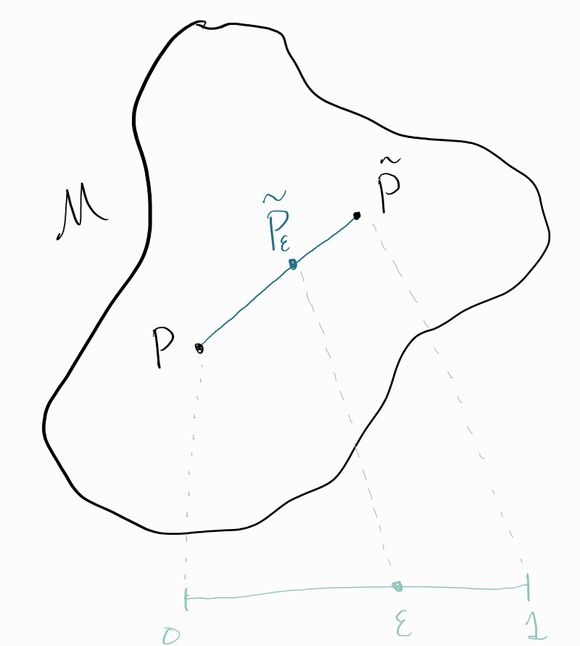
Although this intuitive description makes it clear that a path has a “start” and an “end”, both of which are distributions, what we want to do is name every single distribution along the path too. For example, let’s say we get only halfway from to . Where have we ended up?
The most convenient way to describe the full path is to think of a value that indicates how far along we are. We’ll use the notation to denote the distribution that’s -distance along the path (sometimes you’ll see referred to as the “perturbed” or “fluctuated” distribution). So means we’re at the start of the path () and means we’re at the end (). Our question in the previous paragraph was: where are we if , or for any general value could take?
Let denote the probability density function (evaluated at a point ) for the distribution . We’ll define points along the path to be distributions that have the corresponding densities . This is called the convex combination of the densities and .
Knowing the start and endpoints and that the distributions in-between are convex combinations fully defines these intermediary distributions. For example, if we want to know what the probability is that for a distribution on our path , we could compute
Or, more generally for any event , we could compute . This should also clarify to you that the true probability of a particular event often changes as we traverse the path. But that makes sense if you remember that each distribution represents a different “world” or “universe” in which things are different. What’s interesting about the idea of a path is that we’ve taken some infinite subset of distributions in our model and “lined them up” such that the probability of any given event changes continuously (linearly, in fact) as we move from distribution to distribution.
The full set of perturbed distributions is what we formally call our path “towards” . Since this set of distributions is necessarily a subset of our model , paths are sometimes also called submodels. Moreover, this set of distributions is one-dimensional and therefore is even parametric! If you tell me the one parameter (and and are fixed and known), then I can tell you everything there is to know about . Since paths are parametric models with one parameter sometimes they are called one-dimensional parametric submodels. We generally prefer the intuitive term “path” over the more abstract “one-dimensional parametric submodel” but both are used in the literature.
Differentiable path: technical definition
What we're really interested here are paths that are differentiable in quadratic mean. Specifically, let be some (ordered) set of distributions that we call a path. We say this is a differentiable path if it is differentiable in quadratic mean (DQM), which means that there is some function such that
Where and are the -densities of and . The function is then called the "score" of this path and it must be that (a zero-mean square-integrable function).
This definition actually does not require a dominating measure because for any sequence along the path we can construct a dominating measure using a convex combination of the countably-many measures along the path.
Under some differentiability conditions we have that so this is a useful tool for intuition.
There are restrictions on what can be a path. For there to exist a "legal" path in a direction , we need there to be small enough so that . In other words, paths aren't allowed to immediately take us out of the model space. We have to be able to walk at least a small distance in that direction before we leave . It doesn't make sense to have a path that leads us right off of a cliff into nothingness.
Radon-Nikodym, densities, and change-of variables
There is a very important theorem in measure theory called the Radon-Nikodym theorem that easily lets us transform between integrals under different measures if a certain condition is met. For instance, pick a function and consider the new measure defined by . Roughly speaking, it's clear this is a measure because it also maps sets in to numbers. The Radon-Nikodym theorem says we can also go the other way a lot of the time. if you make up a measure , we can always find its corresponding such that as long as one condition is satisfied: must agree with on what the sets of measure zero are. Specifically, must imply . To describe this we sometimes say that dominates , or that is absolutely continuous w.r.t. , or just . We call the function corresponding to its density w.r.t. . But remember, if we don't have absolute continuity, there is no density.
The great thing about densities is that they allow for a very simple change-of-variables formula when integrating with measures. Since but also , the two right-hand-sides are equal. So we can compute at least this one integral w.r.t. by computing the corresponding integral w.r.t. and vice-versa. More generally, the following holds:
if is dominated by and has density , then .
Score Functions
So far we’ve indexed the paths starting at a distribution by which distribution they end up at. But that’s sort of like giving someone directions from San Francisco to Seattle by saying “start at San Francisco, then go to Seattle”. Technically correct, but maybe not so useful. Instead, we might want to say “start at San Francisco, then go north”. Instead of describing the endpoint, we’re now giving a direction to go in.
It turns out that we can define such “directions” in a model space too. For somewhat arcane reasons, these directions are called scores. A score is a function that indicates a “direction” (like “north”, or “south-southeast”). In two-dimensional space (e.g. surface of the earth) we only need a limited vocabulary to describe directions, but since the statistical model is generally infinite dimensional, the object that represents direction is accordingly more complex. But the idea is the same: if you give me a path from A to B, I should be able to tell you which direction B is relative to A.
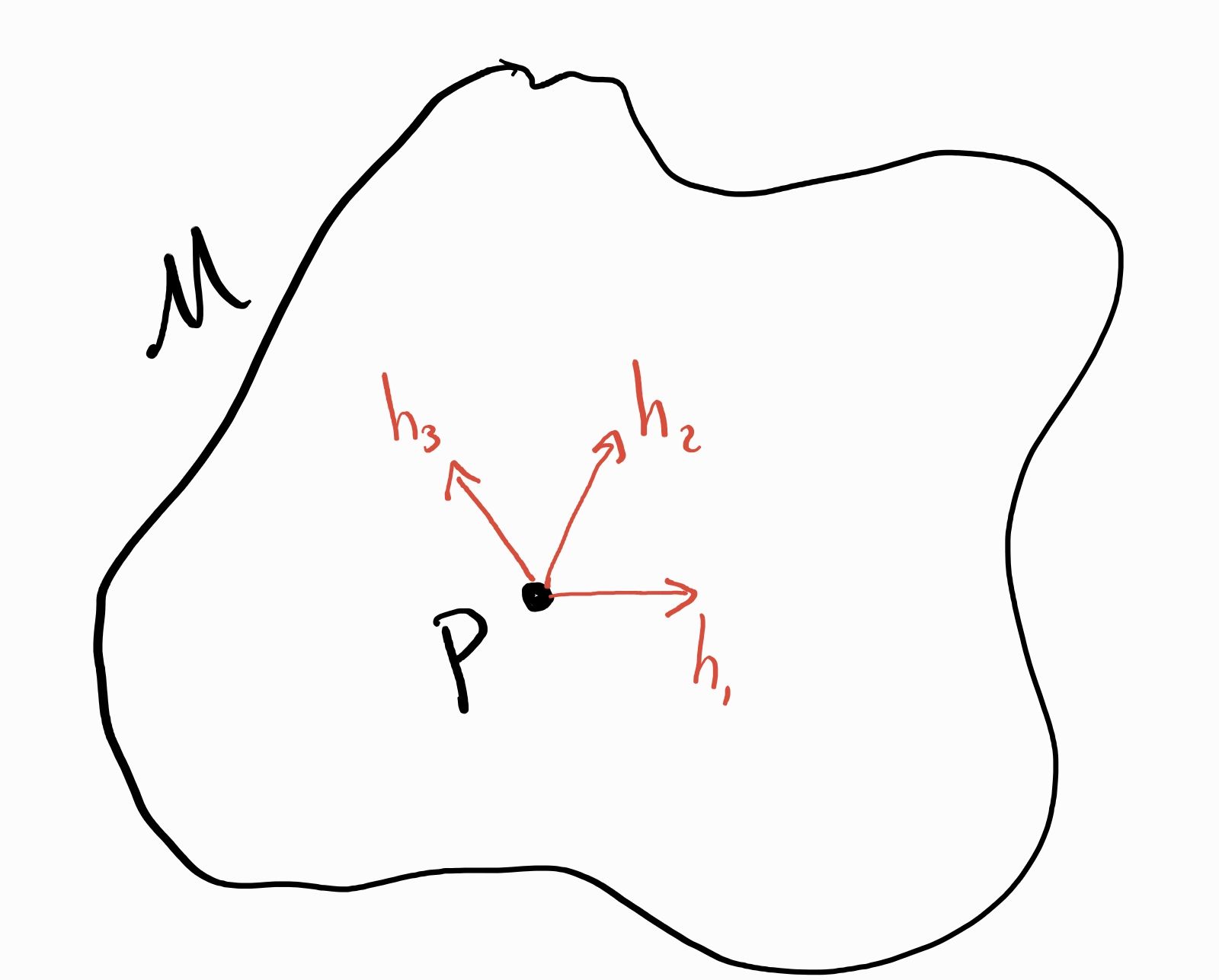
Each score corresponds to a "direction" for a path. It might help to think of as a 3D “blob” here. In infinite dimensions, there are an infinite number of “axes” we might move along.
The technical definition of the score corresponding to a path going towards is just the rate of change of the log-likelihood at . Formally,
It’s probably not immediately clear what this definition has to do with the notion of “direction”, so it might help to consider an example. Let’s presume and let for all . Now define the destination (and 0 elsewhere). What is the score for this path? Using the definition and taking the log and derivative with respect to gives
which you can think of as the vector in 3D space. In other words, you want to move the density in the “direction” to eventually get to the point . That makes sense! The probabilities at the endpoint density are greater at and less at the values 2 and 3 relative to the starting density, so you can see how the direction given by this score suggests that result. If you repeat this exercise with any other endpoint distribution over you will see a similarly intuitive result. This example is simple because takes discrete values, but the intuition is the same when is continuous or even a vector of variables. You just need as many “coordinates” as there are possible values of to describe the direction. Thus the function which maps from any to some number that you can think of as the coordinate for that particular “axis” .
If you do a little math using the change-of-variables formula (assume and are both densities w.r.t. some other dominating measure), you can come up with a definition for the distributions along the path that depends on the score instead of on the destination . This definition is a little less intuitive, but more mathematically useful: . Or, using densities, . We’ll use this version of the path definition many times in the sections that follow.
Any way you slice it, you can still think of the score as a direction you can move in the statistical model (instead of using to define the path). Therefore the set of all paths at is 1:1 with some score function . One path, one score.
Like the influence function, score functions must satisfy . This has to be the case or else the elements of the path won't be a probability distributions because they won’t integrate to 1! That's easy to prove from the definition. This restriction will come in handy many times down the road. We will also impose that scores have finite variance, and of course, that they correspond to a “legal” path.
Back to Regularity
Now we can return to our task of creating a definition of regularity that enforces robustness to distributional shifts. It might look a bit convoluted at first but bear with me.
Pick , some sequence of distributions (which goes to ) along a path. Let denote the empirical distribution of samples drawn from the perturbed distribution . An asymptotically linear estimator is regular if and only if, for all such such sequences we have
Where is some fixed distribution that doesn't depend on the choice of path .
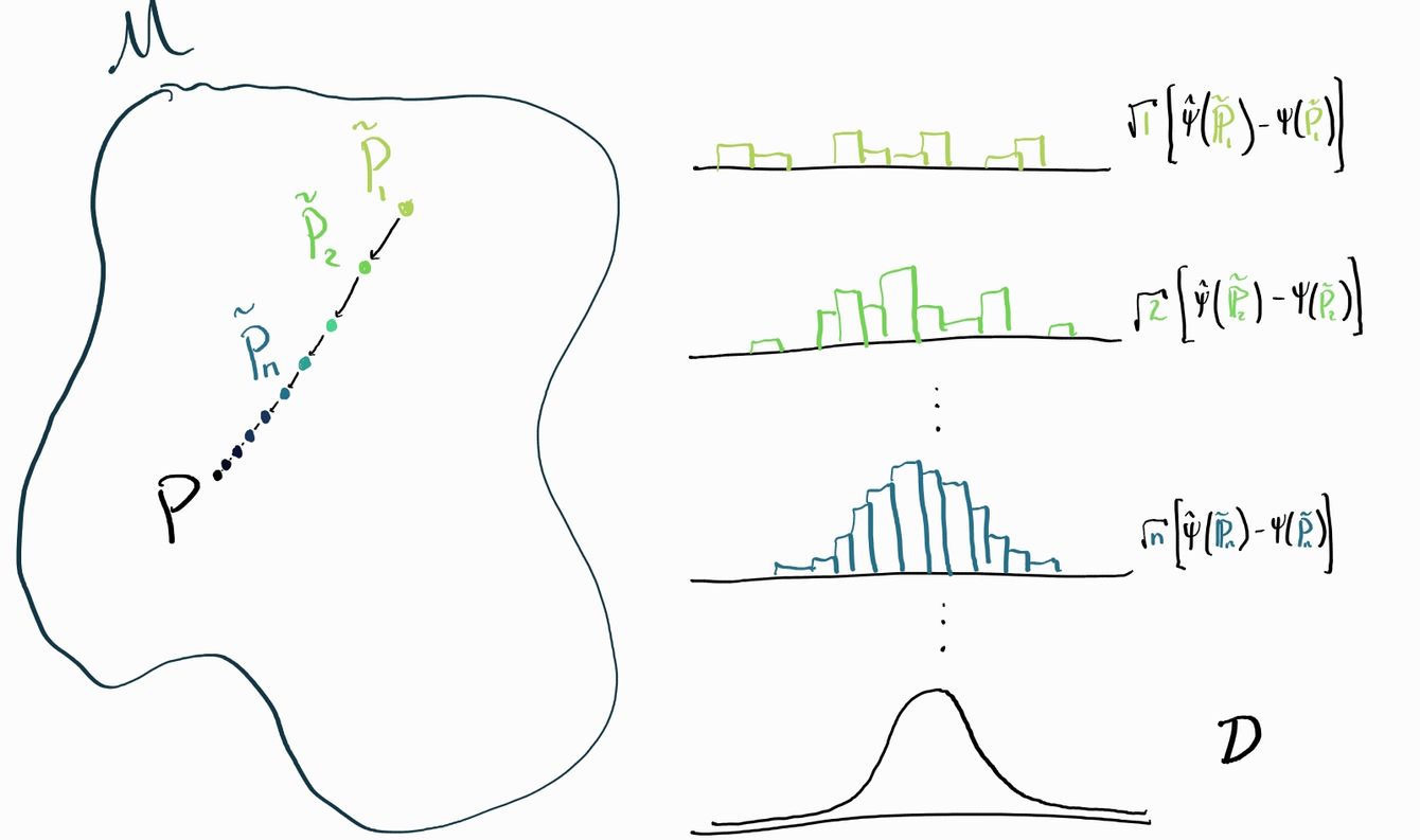
For an asymptotically linear estimator, if we choose the trivial path (where we stand still at ) then by asymptotic linearity we know . Think about it this way: the standard definition of asymptotic linearity just says that our estimator tends towards a normal distribution when we hold fixed and is based on draws from . Now we're saying that our estimator still tends towards the same normal even if instead of drawing from we draw from any sequence of distributions that goes towards quickly enough (but never reaches it!).
You should see this as a sort of "smoothness" or "continuity" condition that holds simultaneously on the mappings and over the model space (and the space of empirical measures that come from distributions on ). Imagine if it were possible to change the distribution an infinitesimal amount such that the parameter experienced some kind of drastic discontinuity. Then it would be impossible to satisfy the condition above because no matter how close we get to with we'll never be able to get within an arbitrarily small distance of . That would make it impossible for there to exist a regular estimator for that parameter (which does happen). On the other hand, imagine that the parameter changes smoothly but that the asymptotic behavior of the estimator (minus truth) doesn't. That's exactly the case for weird estimators like Hodges' Estimator. Then we'd have a situation where we could have valid inference under a distribution but if we tweak that distribution by some infinitesimal amount then all of a sudden we have no idea what the sampling distribution of our estimator is. That's exactly what we're trying to avoid, and that's why we need regularity.
Non-RAL Estimators
Both asymptotic linearity and regularity seem like sensible conditions at face value, but you might wonder whether there are actually some non-RAL estimators that are useful. It depends on what you mean by “useful”, but at least from the perspective of efficiency (minimizing the asymptotic variance; more on this in the next section), the answer is thankfully no.
We’ll start by addressing regularity: if we were to include non-regular estimators, how much better might they actually perform in practice if we were willing to tolerate their idiosyncrasies? For parametric models there is a result that says that any estimator that's more efficient than the best regular estimator can only be more efficient on an infinitesimally small part of the model space. That means we're not missing much of anything so there's no need to worry. In general nonparametric statistical models there isn't an equivalent result because it's less clear how to characterize the "volume" of a particular subset of distributions but the general intuition should be the same. Non-regular estimators typically only excel for a very small, specific set of distributions and outside of those they behave badly (recall our stupid estimator ).
What about asymptotic linearity? For this we have a result called the Hájek-Le Cam convolution theorem (theorem 25.20 in vdV 98) that says that the "best" (most efficient) regular estimator is guaranteed to be asymptotically linear. So if we’re already comfortable with restricting ourselves to regular estimators, we’re not losing anything useful by further restricting to RAL estimators.