In the previous section we learned that the canonical gradient is also the influence function of the most efficient RAL estimator (the efficient influence function, EIF). So, if we want to know what that estimator is (so we can use it!), the first step is to derive the canonical gradient of our statistical estimand in our statistical model. Since the point of doing this is to arrive at the EIF, we typically just say we’re “deriving the EIF”- it’s the same thing either way.
Knowing the relationships between the tangent space, pathwise derivative, etc. etc. in abstract generality doesn't immediately tell us what the EIF is for any specific problem. Basically, we know in theory what it is. But, given a particular statistical model and parameter, how do we actually find it? There are many ways to do this.
Things are typically easier in the fully nonparametric (i.e. saturated) setting. Since there are no restrictions on the tangent space, we can “move” in any direction and that ends up making it easier to derive the EIF. We’ll tackle this case first. There are a few tricks we’ll go over to make this even easier.
When the statistical model is semi-parametric (i.e. non-saturated) things are a harder because there are certain directions we can’t go without departing the tangent space. That makes the math more hairy. Thankfully, due to the factorization of the tangent space, there is a simple-enough method that works in most practical cases.
That said, no one method works for all models and estimands. If you’re doing something very different from what’s already out there you might need new and interesting math!
Before we get to any of that, though, we’ll lay out some generic algebraic tools that will help us build up complicated EIFs from simpler ones.
Gradient Algebra
Sometimes your statistical parameter can be expressed as a fixed function of another statistical parameter, or as a sum of two other statistical parameters, etc. In these cases, it's often easier to find the canonical gradient of the component parameters and then combine them to get the canonical gradient for the original target parameter. Thankfully, it's really easy to do that!
The trick is to realize that the pathwise derivative (for a valid path given by ) is just an ordinary unidimensional derivative for a function of . In brief: . So we can directly apply all of the relevant results from undergraduate calculus: the chain rule, addition of derivatives, etc.
We’ll go through the chain rule as an example. Imagine that you know the canonical gradient for a parameter but what you're really interested in estimating is the quantity . Well, check this out:
This looks intimidating but each step is a something we're already familiar with so it's just about putting it together. At the end of the day, what we've shown is that the function is exactly the Reisz representer for and is thus by definition the canonical gradient of . Note that multiplying by the constant is a linear operation so we can't have left the tangent space (which hasn't changed) and somehow obtained a non-canonical gradient. We therefore have a simple formula (effectively the chain rule) to compute gradients for functions of parameters.
It helps to think of an “EIF operator” for a given model that takes a parameter and returns its efficient influence function . We can write out a few useful algebra rules this way:
We’ll call this “gradient algebra”- it’s a generically useful set of tools that we can use to build up canonical gradients from simpler pieces, the same way we can use the chain rule, etc. to build up complex derivatives from simpler ones. We’ll see some examples in a little bit.
Saturated Models
Life is generally good when our model is fully nonparametric. There is only one influence function, and it’s the efficient one. All we need to do is to find it.
The material in this section closely follows and condenses Kennedy 2022 and Hines 2021, though the methods have been around for much longer!
Point Mass Contamination
The trick most people use in this setting is called point mass contamination (or sometimes the Gateaux derivative method). The idea is to 1) pretend that all the variables in your model are discrete and then 2) to consider a particular kind of path where the "destination" is a distribution that places all of its mass at some point (I'll use to notate such a distribution). In other words, this distribution enforces and the probability that takes any other value is 0. We can therefore think of the path for small as the distribution "contaminated" with just a little extra mass at the value .
Because our model is saturated, we can pick any point and get a legal path of this type. If our model were not saturated at , then there would be no guarantee that for some given a path like this wouldn't immediately take us outside the model space.
Let the score of such a path towards a distribution be denoted . For paths of this type, we can argue that the value of the influence function at the point is given by the derivative of at 0 in the direction of the score . Or, formally (and dropping tildes): . This is extremely convenient! All we have to do to get an influence function is brute-force compute the pathwise derivative of our parameter along paths defined by point mass contaminants. And since there’s only one influence function, if we find one, we’ve found the efficient one.
Proof of
Recall that our definition of the score and path is . The left-hand side is equivalent to and we can exploit our change-of-variables formula to give (as long as , else we lose absolute continuity). Now by the zero-mean property of and linearity of the integral. Thus . The definition of the path in terms of a convex combination of CDFs implies that In the limit as , so by the portmanteau lemma . Moreover, clearly in that same limit. So we have
If is a point mass at , then the integral on the left-hand side here is exactly and . Thus (dropping the tildes). Finally, by our central identity for influence functions, as desired.
Why is it called an "influence function"?
When we first presented influence functions we weren't in a position to explain why they have that name, but now we are! In a saturated model, our arguments above show that for discrete distributions. Using its definition we can expand that derivative as follows:
so what tells us is how much the parameter changes if we add an infinitesimal amount of probability mass at the point . Or, you might say, it is the "influence" that the point exerts on the parameter (at ). That explains the name!
We started out by assuming that our data were actually discrete, so we now have to actually go back and check that the influence function we derived still works in the original model. But this is much easier once we have our candidate: just compute and and check the two are equal for arbitrary in the tangent space .
The whole procedure may seem slightly abstract at the moment but we will see examples shortly. You also don’t have to worry about doing this manually most of the time because you can use gradient algebra to build up your result from the examples provided here!
Example: Mean
Consider the estimand where can have any distribution in a nonparametric model. What’s the efficient influence function?
Point Mass Contamination
First, start by pretending is discrete and only takes values in some set , with probability mass at each point. Then the formula for our estimand is .
Now let’s add a tiny little bit () of mass to a particular point to get a new probability mass function: . Technically this isn’t a probability mass function anymore because the probabilities don’t sum to 1 but we can ignore that: all of this is a heuristic to get us a candidate influence function. Now let’s compute our estimand for this perturbed distribution:
Recall our definition . All we have to do to compute this is take the derivative w.r.t. of the right-hand side above and then set . We get:
This is typical in EIF derivations of this kind: we end up with a term that is the estimand itself (in this case ) and some other terms where the indicator function at cancels out all of the terms in the sum over except for the term at .
Thus we arrive at our candidate EIF:
Checking the Candidate
Now we can check that for any our central identity is satisfied:
From the left:
More generally…
And from the right:
Why does having a candidate EIF make this easier?
Consider the derivation above. Working from the result on the left-hand side we could have noticed that because and then proceeded backwards up the derivation on the right-hand side. That would have gotten us our influence function without ever supposing a candidate.
The problem is that this is a “clever trick” that is really only obvious in retrospect. If we were working from the left-hand side, how would we know to subtract zero in the guise of There are a million other things we might have tried if we didn’t have the right intuition from solving a lot of these problems in the past. Moreover this is a very simple example- in the general case the proof might involve some very unintuitive techniques. Basically: if you don’t already know where you’re going, it’s very hard to get to the right answer.
On the other hand, with a candidate EIF we can just plug-and-chug from the right-hand side and meet up in the middle. No creativity or special intuition required.
Thus we are done and have proved that is the EIF for in the nonparametric model. You may notice this is exactly the influence function for the sample mean estimator, which shows it is nonparametrically efficient.
Example: Conditional Mean
Consider for some discrete variables and and a given value . As in the previous example, we can express this estimand as . The steps will be the same as before: define as the point-mass contaminated version of , compute the derivative of w.r.t. , then set .
Here we can define
Plugging this we can compute and take the derivative. I’ll spare you a few lines of algebra (see Kennedy 2022 if you need it) and tell you that what we end up with is
You can verify for yourself that this influence function still holds if is allowed to have an arbitrary (non-discrete) distribution by following the same steps from the example above.
We can also slightly relax the restriction on to allow arbitrary distributions that have nonzero mass at the point . If there is no mass at , the above influence function is undefined. Indeed it is known that the general conditional mean is not a pathwise differentiable estimand so this makes sense.
Building up Influence Functions
This point-mass contamination strategy works perfectly well for complicated estimands but it can take a bunch of algebra (see, e.g. Hines 2022). Instead of reinventing the wheel every time, it’s often easier to use our gradient algebra tricks to build up a complicated influence function from simpler component parts like those in the examples above.
So far we have EIFs for the mean
and for the conditional mean :
Let’s put these together with our gradient algebra rules in an example.
Example: ATE in an Observational Study
Here we're interested in the general nonparametric model for an observational study with an outcome , binary treatment , and vector of arbitrary covariates . Our parameter of interest is the statistical ATE
Where .
By the linearity, we can get the EIF of by taking the difference of the EIFs of and . So let’s figure out what is, keeping generic.
First, pretend our variables are discrete so . Now use the sum and product rules:
We have an expression for the influence function of because that’s just a conditional mean. We also have the influence function of because we can write . The term is just a particular random variable so we can directly apply our result for the influence function of a mean. As a result:
In the last line we used the fact that and we defined the propensity score . As often happens, we collect a term that turns out to be equal to our estimand: .
This holds influence function holds for discrete data. To check the candidate works for general distributions the trick is to “factorize” the generic score using the tangent space factorization we discussed in the previous section. The details involve some algebra, which you can check at your leisure.
Checking the candidate
We’ll check for since the proof for is the same. From here on we’ll omit the subscript and just write for notational brevity. First, we write the directional derivative for and a general
where the factors of of will depend on - see the section on tangent space factorization on the previous page.
For the covariance of our candidate EIF with general we have:
Since our distribution factorizes , we can write for an arbitrary score. Thus:
What we’ll do is show that each of the vertically stacked terms are equal to each other. I’ll show you in some detail for the terms but I’ll just give you the result for the and terms and leave it to you to verify the algebra by using the special properties of the scores in each of these subspaces.
For the terms:
For the terms: verify that
For the terms: verify that
Since all three sets of terms are equal, this completes the proof that is an influence function for . Thus we have the same result for the ATE because of gradient summation. Since the model is saturated, this influence function is the only one and is therefore the EIF.
Non-Saturated Models
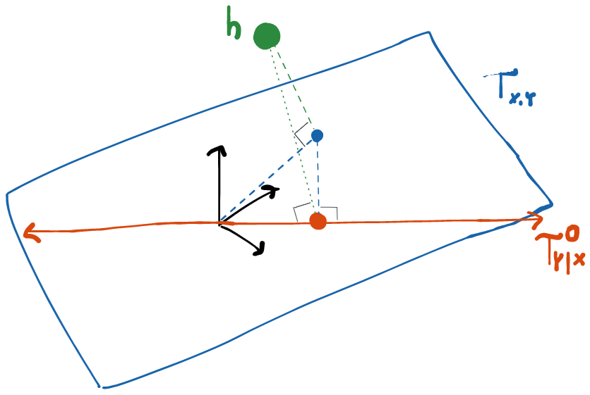
If we have a tangent set that is not all of things get a bit trickier. Here we’ll discuss what’s most often called the projection approach.
The idea is to first find an existing estimator that is known to be RAL and figure out its influence function . Then, taking advantage of the geometry of the problem, we know that the projection of onto the tangent space is the EIF. In this case, finding the EIF is just a matter of computing a projection in . Note that this approach does not apply if the tangent set is because in that case there is only a single valid influence function. Therefore if we had an existing RAL estimator, it would already be efficient.
By "projection" what we mean is the mathematical decomposition of an element of a vector space into a sum of an element of a particular subspace and a vector orthogonal to that subspace. The properties of Hilbert space guarantee that every element has a unique projection onto any given subspace (see: projection in Hilbert space). In the finite vector spaces you're probably used to, calculating projections can be tedious, but it is relatively straightforward vector algebra. In there isn't a general purpose formula given an arbitrary subspace. Thankfully, however, there are a few for the kinds of subspaces we're usually interested in. To wit, we'll consider two kinds of specific subspaces. Imagine our data has two components and (i.e. ) so the possible scores are zero-mean functions .
One important subspace are the functions where , i.e. the functions that just depend on . We'll call this subspace . We already saw a subspace exactly like this come up in the example in the previous section. Let denote the projection of onto a subspace (other authors prefer notation like , etc.). It turns out that:
The notation is a little confusing, but what I'm trying to say is that when you project the function of two variables onto this space you get back a function of just one variable.
The other important kind of subspace that we'll consider is . In words: we're talking about the space of functions that have mean 0 when conditioned on any value of . We also saw a subspace like this one come up in the example above. Once again we have a handy formula:
Here the resulting projection is still a function of both and so I've omitted the explicit notation of the arguments.
You should verify both of these identities by checking the two properties of projections: and .
We can now combine these two formulas. Imagine that we have data of the form and we want to project a function to the space . The functions in this subspace only depend on and so first we need to use our first identity to project down to a function of just and . Then we can use the second identity to project the result into the space of functions where the conditional expectation on is zero. The result is:
This is facilitated by the fact that (i.e. we average over , then , so all that's left is ).
Example: ATE in a Randomized Trial
Let's go back to our running example. In the previous section we derived the tangent space for . We'd like to find the EIF of the ATE in this model.
We know that this model space is not saturated because any probability distribution in it has to satisfy the known treatment assignment mechanism. We'll therefore have to use the projection strategy to find the canonical gradient.
Our overall plan is as follows:
Find the canonical gradient for :
Start with a known RAL estimator of
Derive its influence function
Project that influence function onto the tangent space we found previously (this is the hard part):
Project onto each tangent subspace
Sum the projections
Combine the canonical gradients for and to get the equivalent for
First things first: do we know any RAL estimator of ? It turns out that we do: where is the known randomization mechanism. This is the inverse-probabilty-weighted estimator (IPW) of the mean of conditioned on . For a trial with simple randomization this reduces to a difference of means in the two treatment groups.
It only takes algebra to check that this estimator is asymptotically normal: just subtract from both sides, multiply by , and pass the constant through the sum to see that
By putting it in this form and comparing to our definition of asymptotic linearity we've managed to pick out the influence function . It's also possible to prove that this estimator is regular. One way to do that is to essentially repeat the arguments made in the proof of our main theorem of why influence functions for RAL estimators must satisfy for all , except in reverse: for regularity to hold, we need precisely to show that this identity holds for all scores in the tangent space.
Let's project the influence function we just derived above into the tangent space we previously identified:
Our strategy will be to project into each of these component subspaces and then take the sum. Thankfully, these subspaces are exactly of the form we discussed above, so we can use the projection identities we posited above (and which you checked, right?). Computing these, we get that
To obtain these results I've just applied the identities in the section above and introduced the notation . The rest is just calculating conditional expectations. Please try this yourself and make sure it makes sense to you!
Now we sum to obtain .
This proves the perhaps surprising fact that the canonical gradient for the average treatment effect in an observational study is the same as it is in a randomized trial if one is not willing to make any distributional assumptions about the data-generating mechanisms (aside from the treatment assignment in the RCT).
The important difference you should notice, however, is that this canonical gradient is the only gradient in the nonparametric observational study model, whereas for RCTs there is a whole space of gradients. That has the immediate implication that there are many RAL estimators one could use for an RCT (only one of which is efficient), but there is only one valid RAL estimator (up to asymptotic equivalence) in the observational setting.
Alternative proof exploiting orthogonal decomposition of tangent space
What we'll do instead of finding something to project is actually quite clever and leverages the fact that we've already figured out the canonical gradient for an observational study. Let's start with some facts that we know: (1) we can write any score in as a unique orthogonal sum since those two tangent subspaces are orthogonal, and (2) because the canonical gradient in the RCT model is in the RCT tangent space, which is orthogonal to .
Now let's calculate the pathwise derivative of in the direction through the observational study model. Our hope is that we can somehow end up writing the pathwise derivative as an inner product between and some function, which must then be the canonical gradient.
Because the pathwise derivative is a linear function of the score, we can break it up as follows:
The first term is nothing but the pathwise derivative of in the RCT model for which we already have the canonical gradient . So we can represent that term as . But by our fact (2), this is equivalent to . Adding inside the expectation does nothing because it's orthogonal to the RCT canonical gradient. So now we've got
Now we'll brute-force calculate the second term:
Let's drop the subscripts for the moment. We also have that
Because is in the tangent space of densities , the only way to distribute that term to get three legal densities of the form above (that factorize ) is to put the term into . What this shows is that walking along any paths that are in actually doesn't change or . The fluctuated density has the same marginal density for the covariates, and the same conditional density for the outcome given treatment and covariates. The only thing walking along paths in can change is the treatment assignment mechanism. This should make sense to you because these are exactly the paths we are forbidden to walk if we're constrained to the RCT model in which we must hold the treatment assignment mechanism constant but we're allowed to change anything else.
Going back to the expression for the pathwise gradient, we can show using iterated expectations that where . However, by the argument above, and so, in fact, . In words, we've shown that moving along paths in does nothing to the parameter . Therefore and we can plug that into our calculation of the pathwise derivative for general :
Since we've succeeded in expressing the pathwise derivative of this parameter along any path as an inner product between and a function we have that this is in fact the canonical gradient of the conditional mean in the nonparametric observational study model .
Other Methods
Combined with gradient algebra, point mass contamination and projection are two very useful strategies for deriving efficient influence functions.
Unfortunately, there are some rare cases in which they don’t work. For example, if the tangent space factors, but not orthogonally, it becomes much more difficult to find projection (though methods do exist for doing this). Another common approach is to find the influence function in the full-data (causal) model and then figure out a way to map it to the observed data (statistical) model (see Tsiatis 2006 for details). Also, in rare cases, the tangent set isn't even a full space (i.e. instead of being a hyperplane, it's some sort of "triangle" in that hyperplane) and this can also pose difficulties.
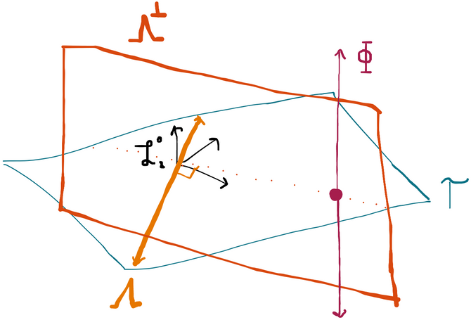
Nuisance Tangent Space
In many texts and resources you'll find mention of something called the "nuisance tangent space". This is a tool that is sometimes helpful in characterizing the set of influence functions, but it is by no means always necessary. Indeed, we don't use it in any of the examples in this chapter. Historically it played a much larger role in efficiency theory, which is why you'll see it mentioned a lot in the literature.
The definition of this space that you'll see most often relies on a semiparametric construction of the model, where every distribution is assumed to be uniquely described by a finite-dimensional vector of parameters that are of interest and some infinite-dimensional vector of parameters that are not of interest. For example, you might consider a model like . When you have this kind of construction, you can calculate scores for each parameter and define the the nuisance tangent space as the completed span of the scores for .
I think this construction is sort of artificial. The definition I like more is that the nuisance tangent space is the completed span of all scores such that . This more general definition is due to Mark van der Laan. The nusiance tangent space is usually denoted or , which is a subset of . It's immediate from our definition that any influence function is orthogonal to any element of . If we denote the orthogonal complement of using the notation , then we have that . Knowing this is sometimes useful in deriving the efficient influence function, but we don't use that fact in any of the examples in this book.
None of this is anything you should worry about unless you plan to work on esoteric new parameters and model spaces for which the canonical gradient has not yet been derived. You probably won’t come up against anything that required tools beyond what’s in this section, but mileage may vary!