Now that we have causal models and estimands and understand how they are different from statistical/observable models and estimands, we can start to see the problem we have with causal inference. We're trying to infer a causal estimand that answers some kind of "what if" question. But we don't get to see data from the distribution , we only get to see data from a different distribution . We’ll explain what this is in a second. Therefore we can only do inference on estimands of the observable (statistical) distribution , i.e. , which is not what we care about!
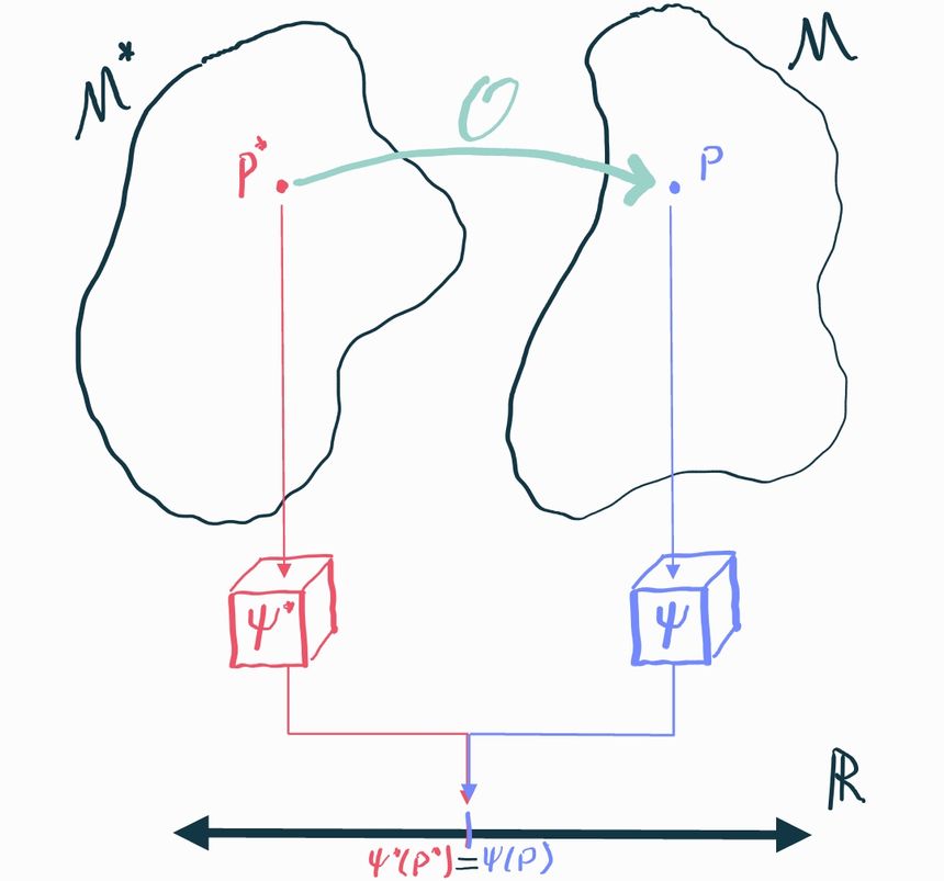
We will call the causal distribution and we’ll call the corresponding statistical distribution. It’s called this because, since we can observe data from it, we can bring all the tools of statistics to bear on it. Sometimes we’ll also refer to as the observable distribution, which perhaps is a bit clearer.
Since it's only possible to infer stuff about , the best we could possibly hope for is that there is some aspect of that happens to tell us about the aspect of that what we actually care about. Specifically, we have to prove that there is some statistical estimand such that . If we can show that, then any inference we can make about will immediately translate to and we're in business because we know how to do inference on : that's just an ordinary statistics problem.
Unfortunately this is not always possible, which we'll show by way of an example. Let's start by presuming that encompasses any possible joint distribution between . For simplicity, consider the case where there are no measured covariates so we only have to care about the joint . Let's consider two different possible distributions in this causal model and calculate their ATEs :
These distributions are actually deterministic: draws from are always , while draws from are always . Now let's calculate the corresponding observable distributions using the relationship . In both cases, we get . Therefore .
But this is a big problem! and are identical, but we need to use them to make inference about in one case and in another. There is no way we can define some statistical estimand that satisfies and because but .
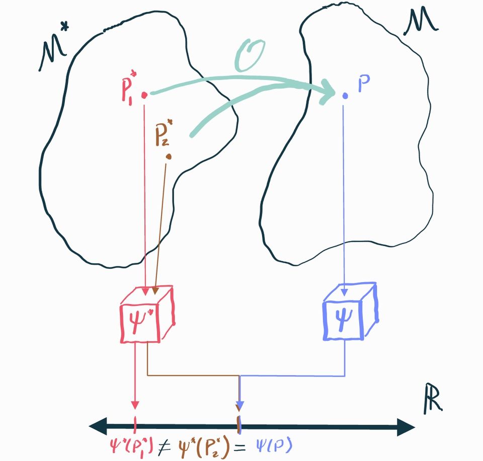
This example shows us that there are cases where there is no statistical parameter that uniquely identifies the causal parameter . We need to impose additional structure on the causal model to fix this.
Identifying Assumptions
The example above highlights the general difficulty with identification: there are generally many causal distributions in the causal model that could map to the same observable distribution. If these different causal distributions have different values of the causal estimand, we're screwed because there is literally no way to tell them apart based on what we can see.
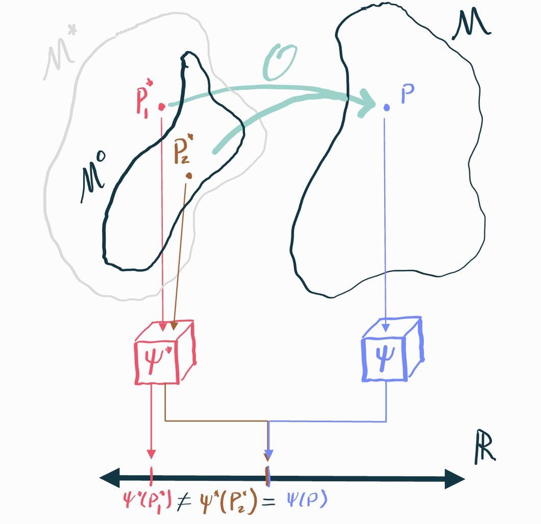
If we are less ambitious, however, we can make progress. Since the problem is that causal distributions with different causal estimands "collide" into the same observational distribution, we might be able to say something in cases where we can rule out those collisions. In mathematical terms, we can restrict our causal model to be smaller: let's say some subset . If we can guarantee that, in fact, , then we just need to prove our identification result holds over all distributions in the smaller set rather than the larger set . If the only relevant collisions are between distributions that are in and those that are not, then we can effectively rule them out entirely if we know that the truth is the one that's in .
We call the assumptions that define what distributions are allowed in identifying assumptions. Since these assumptions gate what we consider to be possible and impossible, they must be argued for on the basis of domain knowledge. Identifying assumptions are always fundamentally untestable (i.e. the data you observe can neither support nor reject them) because they pertain to aspects of the causal model that are unobservable.
Examples
The best way to understand identification is to look at a few examples.
Identifying the ATE in an Observational Study
What are some assumptions we could impose on distributions over so that the ATE is identifiable? And under these assumptions, what exactly is the statistical estimand that identifies it?
Let's think about what our problem was in identifying the causal effect in the general, unrestricted causal model . The issue with the counterexample we gave was that was tied to and in such a way that in the observable distribution we never got to see . That's why we ended up with a situation where .
It turns out this scenario actually captures two assumptions we will need to put on , which are
Unconfoundedness: for each
Positivity: for all ,
we can also recall the definition of our observational transformation , which some authors consider an identifying assumption. However, strictly speaking, this does not restrict to so much as it defines how these spaces are linked to . Nonetheless we can include this for completeness:
Causal consistency:
Before we discuss what assumptions (1) and (2) really mean, let's see how we can invoke them to prove an identification result. We'll start with the causal parameter , the counterfactual mean outcome under treatment .
Our final expression is something that depends only on the observable distribution . We've established that inference about the quantity tells us what we want to know about the causal quantity which is what we really care about. We say that the statistical estimand identifies the causal estimand in the identifiable causal model . From this we conclude that identifies the ATE .
We used all of our assumptions about to prove identification. Unconfoundedness allowed us to condition on after having conditioned on without changing anything. Because of the independence, we know and therefore . Positivity played a more subtle role: the conditional expectation is only well-defined if the conditioning event has positive probability, so you can think of this as a "don't divide by 0" sort of assumption. Lastly, causal consistency let us see that , which completed the proof.
Unconfoundedness and Positivity
We just showed that unconfoundedness and positivity ensure that we can identify the causal average treatment effect using the observable treatment effect. But what do these assumptions really mean? If we can't explain to collaborators (or to ourselves) what the implications of these assumptions are, then we can't assess whether or not they are reasonable to impose.
Let's start with positivity, since it's relatively simpler. for all and means exactly what it sounds like: any individual in the data must have had some positive probability of getting either treatment or no treatment based on what we know about them from their covariates.
There are obvious ways in which this may not be the case. For example, imagine an observational study on the effect of a tax incentive on individuals' savings in the next year. Presume that, by law, the tax incentive is only given to people who make less than $50,000 a year and never to those who make more than that. If we let be income and be the tax incentive, then clearly and , which is a violation of the positivity assumption. Therefore we simply cannot estimate the causal effect that the tax incentive has on savings (even with infinite data!) because it is not identified by the observable statistical treatment effect.
The intuitive reason for this failure is that no matter how much data we gather, they provide us absolutely no information for what happens if someone making over $50,000 gets the tax incentive, or for what happens if someone making under that amount doesn't get the incentive. There is simply nothing we can say about those scenarios without data, unless we want to make further, stronger assumptions.
Unconfoundeness is a little bit trickier, but it's nothing too crazy. just means that all the common causes of and must be contained in . A technical term that we use to describe common causes of and is counfounder. For example, age () is a confounder for knee replacement surgery () and heart attacks () because old age contributes to both knee replacement and heart attacks (regardless of hypothetical knee replacement status). So we we say we assume "unconfoundedness" what we really mean is that we assume there are no unobserved confounders, i.e. we assume all confounders are included in the vector . Other authors use different terms for this assumption, including "ignorability (conditional on covariates)" and "exogeneity", so just be aware of that.
If there were an unobserved confounder such that and then in general this precludes independence between and , even conditional on , because if were to change then both and change together and therefore cannot be independent. Mathematically speaking, means that we must have . In other words, knowing doesn’t tell us help us predict at all if we already have . But if is a common cause of and that isn’t contained in , then generally would help us predict above and beyond because tells something about , which in turn tells us something about that by itself can’t.
As with the positivity condition, it's easy to imagine cases where unconfoundedness is not satisfied. For example, presume we're doing an observational safety analysis to make sure that knee replacement doesn't increase the risk of having a heart attack. Presume we don't collect any covariates and our population of interest includes a variety of age groups. As we already discussed, age is a confounder for knee replacement and heart attacks, so we would not be able to guarantee identification. Even with infinite data, we would not be able to estimate the causal ATE.
The reason this happens is that we end up with disproportionate sampling and no possible knowledge of how to correct for it. In our example study we might see that a high proportion of people with knee replacement also have heart attacks, whereas people without knee replacement tend to have lower rates of heart attack. But this is just because people with knee replacement tend to be older, not because the knee replacement is what actually causes the heart attack. Since we don't measure age, there is literally no way to "control" for this variable, meaning that estimating the causal effect is hopeless.
It's important to realize, however, that even if we did have this variable (and all other confounders, thus proving identification), we would still have to prove that our estimator of choice actually does a good job at estimating the statistical estimand that identifies the causal ATE . In other words, measuring confounders is not enough- we also have to do a good job at controlling for them. For an example where an estimator doesn't do a good job, look back at our section on linear regression in observational studies.
ATE via the propensity score
We already saw that the causal ATE can be identified with the statistical ATE as long as unconfoundeness, positivity, and causal consistency hold. Our expression for the statistical marginal mean was . If we take out the inner conditional mean and name it then we can equivalently say , which neatly shows that the statistical ATE only depends on the two unknown functions and .
Here we’ll show how a different-looking statistical estimand can also identify the causal ATE under these conditions.
Let for ease of notation. We’ll call this function the propensity score (for ). When we usually drop the subscript and abbreviate since .
For identification, again we start with the causal marginal mean:
and an identical argument shows that, more generally, . This quantity is in fact equal to (indeed it must be, by transitivity), but it is independently useful because it suggests a different “natural” estimator.
What do we mean by this? Well, consider the statistical estimand . If we had an estimate of the conditional mean function, say obtained from a machine learning algorithm, then a natural way to approximate the expectation would be to replace it with a sample average. Thus the “natural” estimator suggested by the estimand is . This is called the plug-in or outcome regression estimator. Of course we can’t really say much about the properties of this estimator without some more elaborate argument and knowledge of how is estimated, but all we’re claiming here is that this is an estimator that “makes sense” intuitively.
Now consider the equivalent estimand . Let’s say now say we have an estimate of the propensity score . Again replacing expectation with a sample average, the natural estimator this setup suggests is , which is called the inverse-probability (of treatment) weighted (IPW or IPTW) estimator. Again, to be clear, we can’t say anything about how this estimator actually behaves without additional arguments.
The upshot of all of this is that, just from identification, we’ve found two very different but seemingly reasonable candidate estimators for the marginal potential outcome means (and thus for the ATE) under the same set of assumptions. In one case we’d have to estimate the outcome regression models and in the other we’d have to estimate the propensity score .
ATE in an RCT
We’ve seen that identifying the ATE in a general observational study requires us to assume positivity and unconfoundedness. But what if we’re in an RCT? It turns out that we don’t need any assumptions at all.
What do we know about the causal model ? Since treatment is randomized (let’s say 50:50), we know that for a fact. Therefore the treatment is independent of everything, including potential outcomes . We don’t even need to condition on . That’s unconfoundedness taken care of! Positivity is also satisfied because for any .
What we’ve shown is that the RCT causal model satisfies the identifiability conditions for a generic observational study: . So we don’t need any additional assumptions: the ATE is identified by design: .
This is precisely why RCTs are so valuable. If you’ve randomized treatment, your estimate of the statistical treatment effect is always an estimate of the causal treatment effect. The same is only true for observational studies if you are willing to believe in some identifying assumptions, which are always arguable. You can never be sure you’ve measured every single covariate that you need in order to get unconfoundedness, or that treatment isn’t completely deterministic for some kinds of observations. You have to make your best argument and accept the fact that you might be wrong!
Of course, RCTs are a little more complicated in reality. For example, if subjects drop out of the study, you still have to fall back on other identifying assumptions. That’s why trialists care so much about retaining subjects. Either way, the point is that real-world RCTs are generally not 100% assumption-free. But nonetheless, not having to worry about confounding or positivity bias is a huge bonus.
Identification in an RCT with dropout
The purpose of this example is to show you how dropout is generally represented in causal and statistical models.
As usual, we have our covariates , treatment , and potential outcomes . Now, however, we will add an indicator that tells us whether or not we got to observe the outcome for that subject () or whether they dropped out ().
In our statistical model, we get to observe directly, but of course we can’t directly access the potential outcomes. We can only see , the potential outcome corresponding to the observed treatment. We also have to contend with the missingness: we get to see when , but otherwise we see (or any other arbitrary value we choose to represent NA) when . Thus in total what we observe is .
Since we’re in an RCT we already satisfy treatment positivity and unconfoundeness. But now we have to contend with the outcome missingness too. Let’s consider what would happen if some segment of our population always dropped out. We would never get to see the outcomes from these people, even with an infinite sample. If this group is substantially harmed by the treatment, we would always overestimate our average effect (and vice-versa). So we have to make some assumptions about the relationship between , , and in our causal model or else we can’t identify the effect.
In some cases it’s reasonable to argue that . We call this missing completely at random (MCAR). Following the identification examples for an observational study (above), try to show that the MCAR assumption is enough to buy identification of the ATE in an RCT with outcome missingness. Can you show that the ATE is identified in this setting with an even weaker set of assumptions?
Post-Treatment Variables in an RCT
So far we’ve seen that we can identify the causal effect we’re interested by conditioning the observed outcome on the covariates , which up until now are things we presume to have measured before the intervention happens. The arrow of time thus dictates that could causally affect but not vice-versa. Now we can ask what would happen if were to represent something that occurred after and could be affected by the treatment. In other words, what if we condition on post-treatment variables?
This is a practical and relevant question. Imagine you have a randomized trial (a special case of observational study, really) and in your dataset you have variables that were recorded both before and after the intervention of interest. Our identification result tells us that what we need is the conditional mean of the observed outcome, conditioned on all pre-treatment variables that could affect both treatment and outcome.
But what if we also condition on some post-treatment variables? In terms of the linear regression example from the previous chapter, this would be equivalent to including these post-treatment variables as predictors in the regression. What happens if we do this?
Let’s draw a SWIG to clarify what we’re talking about. First we have the intervention , which when set to gives rise to the potential outcome . Since we’re in a randomized trial, is set by a coin flip so there are no arrows going into it. We also have a post-treatment variable that we call . Since is post-treatment, it also has potential values that would obtain under counterfactuals ! The last thing to notice is that there is an unobserved pre-treatment variable that affects both and . We’ve omitted any measured pre-treatment covariates to simplify the picture.
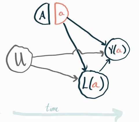
To make it concrete, you can imagine that represents a new drug vs. standard of care, represents the presence of an unmeasured genetic risk factor, is a measure of each subject’s health one month after starting the trial, and is the same measure of their health one year after starting the trial. In this example you should expect that people with the gene () have worse health both a month and a year after the start of the trial relative to people who don’t have that gene. It’s easy to imagine trials where all the genetic risk factors are unknown and thus unmeasured. This is a very realistic example of why unmeasured baseline factors typically exist which would affect both the outcome and other post-treatment variables.
Our idea here is to condition the observed on the observed value (and ) and then average over , same as we did above with . To be clear, is the value we can observe in the real world, not the potential outcomes .
Mathematically, we have the following statistical estimand . Does this identify the causal estimand ?
The answer is no! To get our identification result before, we had to be able to assume that and were independent conditionally on the conditioning variable, which was . If we condition on , though, we don’t get this independence! To see why, consider the structural equations that correspond to the SWIG above:
We’d like to show that , where is the observed value of . Plugging in the above, that translates to
What you should notice is that both and appear in the left- and right-hand sides of the conditioning. Typically, that means that knowing something about when we already know will tell us something about what must have been, which in turns tells us something about . This contradicts the definition of conditional independence.
A concrete example
Imagine that (i.e. half the people in the population have the genetic risk factor). Moreover imagine that (i.e. outcome is deterministic based on gene and ignores treatment) and that is 0 if and if (i.e. the treatment is protective against risk for some time, but then wears off). By definition we can expand and plug in to get .
Now, rewriting with what we’ve obtained here we get . For this conditional independence to hold we would need for . We can easily show this is not the case by writing out the full joint distribution:
Consider the case . From the table we can read off for this case, but we also can see so .
Of course, so the conditional independence cannot hold.
What’s especially striking about this is that and were already marginally independent because of randomization. We have identification without conditioning on anything at all. But conditioning on the observed value of created confounding where there was none. Information was able to leak between and because of !
This is why our identification proof breaks down and we can’t show that the statistical estimand identifies the causal estimand (because it doesn’t!).
The implication is that you should never adjust for post-treatment variables in any way, or do anything that implicitly creates this kind of conditioning (e.g. excluding subjects from a study dataset based on post-treatment factors). This is a well-known source of bias and you can read a lot more about this subject here.
Exploiting Structure
There are generally multiple different overlapping sets of assumptions that you can impose on your causal model to get you identification. We already saw that unconfoundedness and positivity do the job for the ATE in an observational study, but now we’ll see there are also alternatives that depend on having some additional known structure in your data. We won’t get into a lot of the details here, the point is just to show you the diverse kinds of assumptions and causal estimands that you’ll find in the wild. I’ll introduce you to four common identification strategies you should be aware of but there are many more bespoke results out there. Once you understand identification conceptually it should be possible for you to parse a paper with a new identification result.
You should also be aware that people often refer to things like “an instrumental variables analysis” without clearly separating the identification and estimation steps. Here we’ll only discuss what is most important conceptually, which is the identification strategy that takes you from some causal estimand to a statistical estimand. Once you have a statistical estimand, the rest is just statistics!
Instrumental Variables
Imagine that we’re not willing to assume away any unobserved confounding. That is, we have reason to believe that there are factors we haven’t measured that affect both a subject’s likelihood of treatment and their observed outcome. But now let’s also say that we know that one of our (binary) measured covariates (call it ) has an effect on the treatment assignment but couldn’t possibly be affected by any unmeasured confounders. Moreover presume can’t affect the outcome except through the choice of treatment. If these conditions are satisfied we say is an instrument or instrumental variable (IV).
For example, let’s say we’re interested in the effect of maternal smoking cessation on birthweight. Even in a randomized trial, all we can do is encourage the treatment arm participants to stop smoking. This encouragement () doesn’t necessarily mean a person will stop smoking (). However, since we randomized the encouragement, we know is independent from any possible unmeasured confounders. It also seems unlikely that encouragement to stop smoking could affect birthweight via any means other than smoking cessation.
Incredibly, knowing this is almost enough to identify a certain kind of causal effect sometimes called the complier average treatment effect. The complier ATE is just the ATE but within the subpopulation of subjects who would always follow the IV “recommendation”. Usually another assumption is required to get this identification result, for example assuming that can only increase the probability of for any observation. It’s also sort of difficult to interpret the complier ATE (who are the compliers?) so sometimes further assumptions are imposed so that the complier ATE is equal to the standard ATE.
A proof of this type of identification result and a more detailed explanation is given in Baiocchi 2015.
Regression Discontinuity
In some cases, treatment is assigned deterministically on the basis of a singe continuous covariate. For example, perhaps people who make under $100k/year are given a particular tax incentive and those who make more than that are not. How can we assess the impact of this intervention with such a clear positivity violation?
As usual, the key is to either impose stricter assumptions or to be less ambitious in our aims. The idea of regression discontinuity is that observations just on either side of the cutoff are basically comparable to each other. For example, is there really an income difference between $100.001k/year and $99.999k/year? Probably not. Since the treatment is known to be assigned based only on that one variable, all else should be practically equal and we’re essentially in a randomized trial if we only consider observations in a small neighborhood of the cutoff. Under mild assumptions, we can therefore identify a local ATE, even if the population ATE remains unidentifiable. If we’re willing to make more assumption (e.g. constant treatment effect) then maybe we can say something useful about the population ATE.
As with my description of instrumental variables approaches, my goal here is just to give you an idea of what’s out there. There are many, many more details and nuances in terms of how local the effect can be made to be and under what assumptions. You can find a review and more details in Cattaneo 2022.
Difference-in-Differences
Consider a problem where we measure a certain variable in two different groups, then deliver an (nonrandomized) intervention to one of the groups and remeasure that variable in both groups after delivering the intervention. We want to know what the effect of the intervention was on said variable for the treated group.
In a problem-agnostic sense, we can treat the first measurement of the variable as a generic baseline covariate and the second measurement as an outcome and then try to identify an ATE (or ATT: average effect on the treated, defined as ) using the same approach we described above. However, unmeasured confounding could be a concern and we don’t have an instrument we can exploit.
Instead of trying to get at the confounding directly, a reasonable idea is to assume that such confounding could only affect the change in the variable of interest across the two timepoints in a specific way. Specifically, we assume that absent any intervention, the tracked variable in the two groups would have followed parallel trends, conditional on baseline covariates .
Formally, if we let represent treatment and let be the potential outcomes at time , we will assume
A little algebra shows this is enough to identify the ATT of interest, which is .
This overall strategy is called difference-in-differences (DiD) A review and some more details can be be found in Abadie 2005.
Negative Controls
A negative control outcome (NCO) is an outcome that we know cannot be affected by the treatment of interest. For example, if we’re studying the effectiveness of the flu vaccine on flu hospitalization rates, then hospitalization for a traumatic accident might be a good NCO. It’s exceedingly implausible that getting the flu vaccine would cause people to have more accidents.
Similarly, a negative control exposure (NCE) is an exposure that we know could not affect the outcome of interest. For example, whether or not someone had a regular doctor’s office visit in the past three months almost certainly has no causal effect on flu hospitalization.
NCOs and NCEs can both be affected by unobserved confounders. Let’s say certain people have personalities that make them more likely to engage with the healthcare system. That might be measurable via a survey or something, but presumably that’s not information we have so “personality type” is an unmeasured confounder: it could affect someone’s willingness to get the flu shot as well as their willingness to go to the hospital if they get the flu. Our NCO and NCE would also be affected by this confounder because people who engage with the system would be more likely to go to the hospital for a traumatic injury and to go to their regular checkup appointments. In fact, this is required: the NCO and NCE must reflect variation in the unmeasured confounder in order to be of use in this framework.
Formally, let represent an NCE, let be an NCO, and let be some unobserved confounders. Since is an outcome, it also has potential outcomes in the causal model, but now we also have to attend to the fact that there are two different interventions: and . Therefore we write to represent the four potential outcomes and we do the same for our standard outcome . We can now formally write our identifying assumptions:
There are several identification results for the ATE that we can get by combining these assumptions with positivity and one or two mild technical conditions. There are some variations where you don’t even need both the NCO and NCE. Shi 2020 is a great review of these proofs and methodologies.
Proximal causal inference is a broad generalization of this framework that admits many different kinds of variables as proxies for unobserved confounders. Tchetgen Tchetgen 2020 is the right place to start if you want to learn more about that.