A causal model is fundamentally the same as a statistical model in character: it's just a collection of probability distributions that satisfy some assumptions. The only difference is that the causal counterpart of a statistical model has slightly different variables in it which are related to the variables in the statistical model.

This is easiest to understand at first with an example. Consider our interventional study setup where our statistical model consists of data-generating distributions over a vector of covariates $X$, a binary treatment $A$, and an outcome $Y$. When we ask about the effect of $A$ on $Y$, what we're after is a what-if scenario: what would the outcome $Y$ have been for a particular individual if the treatment had been $A=0$? What about if it had been $A=1$? Let's call those two what-if quantities $Y(0)$ and $Y(1)$ respectively. These two separate random variables are referred to as the potential outcomes or counterfactuals. The fundamental problem of causal inference is that we can only observe one of these at a time for each observation: if someone gets treatment $A=0$, we can only observe $Y(0)$. We'll never know what would have happened if they had gotten $A=1$ and vice-versa.

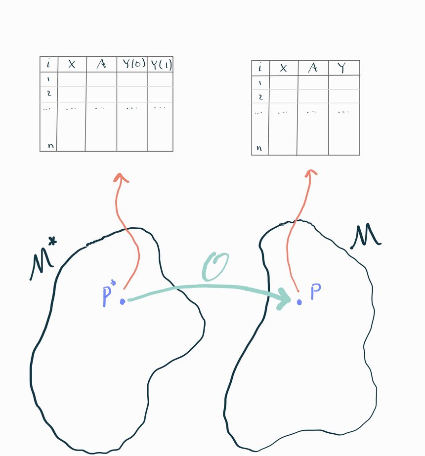
Nonetheless, that's precisely the kind of information we need to answer causal questions. So let's imagine if we could see a dataset that contained observations of both potential outcomes for each observation. Some authors call this the "science table". We can contrast this with the corresponding dataset we'd see in the real world:

Do you see the difference? On the right side we've mashed together the two variables $Y(0)$ and $Y(1)$ into one variable $Y$ that takes the value of $Y(0)$ if $A=0$ and the value of $Y(1)$ if $A=1$. You'll sometimes see this written as $Y = AY(1) + (1-A)Y(0)$. You can also write this as $Y(A)$ with the understanding that $Y(a)$ are two separate potential outcomes and you are choosing which one to observe based on the realized value of $A$.

In general, you might work with data that has a more complex structure than this. For example, what if you're interested in the effect that a combination of two different drugs has on survival? If we presume that people could take either one drug, both, or none, we might define two different treatment variables $A_1$ and $A_2$ that indicate whether each person is taking each drug (e.g. $A_1=A_2 = 1$ indicates both). In this case there are four potential outcomes that might be of interest: $Y(0,0), Y(0,1), Y(1,0)$, and $Y(1,1)$.

In general, there are as many potential outcomes as there are different combinations of interventions of interest. Any variable that you wish to manipulate in a "what-if" scenario is something you should consider to be "an intervention". The number of values it can take (in combination with other interventions) determines the space of potential outcomes. This even extends to continuously valued interventions, like the dosage of a drug (e.g. $A \in [a_l,a_u]$). In this case we can't enumerate all of the infinite potential outcomes, so we typically just refer to them as $Y(a)$. Remember, however, that for each $a$, the quantity $Y(a)$ is a different random variable.

Counterfactual distributions can also be represented graphically. The technology we use to do that is called a single-world intervention graph. The basic idea is the same as the DAGs we saw in chapter 1. Each variable gets its own node, and an arrow connects a variable to another if the former appears in the right-hand side of the structural equation for the latter.

The only difference is that now we have to represent the possibility of intervention, i.e. that $A$ may have its value forced to $a$ and the downstream implications of that. To do that, we split the node for an intervention into two: one that represents the “natural” value $A$ and one that represents the “intervened” value $a$. Nodes subsequent to the intervention are affected by $a$, but not directly by $A$! Notice that the constant $a$ is also not tied to the random variable $A$ because the natural value of the intervention doesn’t typically affect the value we force the intervention to. Nonetheless we place $A$ and $a$ adjacent to each other so that it’s clear that they are related.

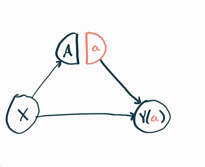
Since $Y(a)$ and $Y(a’)$ are two different random variables, they should each technically get their own node. But for notational convenience we just write $Y(a)$ and understand that the graph we’re looking at is a template where we can replace $a$ with $a’$ throughout, or any other value of the intervention we could be interested in.

Instead of thinking of the observed data as a direct transformation of the causal data, we'll see it's more useful to think of both of these as draws from two separate but related data-generating distributions. We'll continue working with the interventional study example. As we know, the statistical data-generating distribution is the probability distribution that generates observations of $(X,A,Y)$. We'll call it $P$ and say this is an element of a statistical model $\mathcal M$. The causal data-generating distribution is the distribution that generates observations of $(X,A,Y(0), Y(1))$. We'll call this distribution $P^*$ and say it lives in a causal model $\mathcal M^*$.

These two distributions are related to each other: the statistical distribution is completely determined by the causal distribution because of the way $Y$ is constructed from $A$, $Y(0)$, and $Y(1)$. If we want to be very explicit about this we can write the density of the causal distribution in factored form

now we define $p(Y=y|A,X) = p^*([AY(1) + (1-A)Y(0)] =y | A,X)$ and finally we can construct

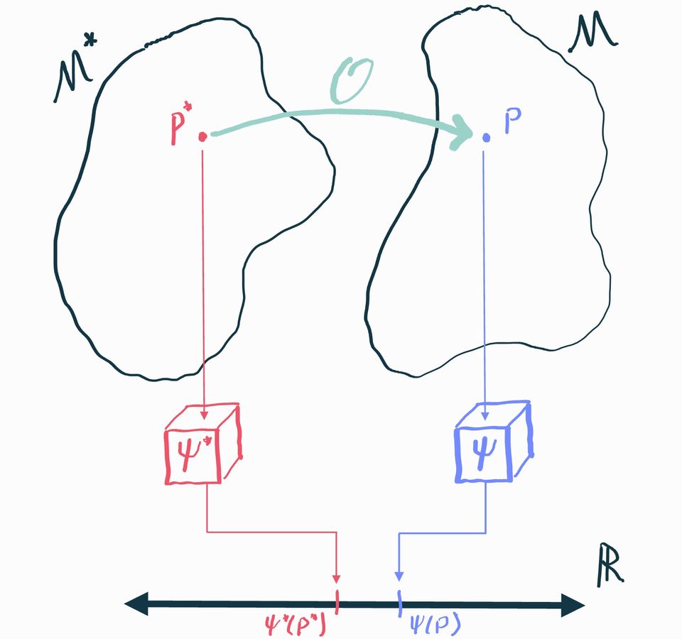
You can think of this as an algorithm that takes any distribution $P^*$ in the causal model $\mathcal M^*$ and produces the statistical counterpart $P \in \mathcal M$. We'll call this the observational transformation, which we can denote $P = \mathcal O(P^*)$

This way of thinking of full-data vs. observable distributions is incredibly powerful and also lets us describe problems where observed data may be missing, censored, or coarsened. For example, consider a randomized trial where some subjects drop out and don't have their outcomes observed. The way we'd describe this is to say that the causal distribution is defined over $(X, A, Y(0), Y(1), D)$ where we've introduced a variable $D$ that indicates whether or not a subject drops out of the study. The observed data we get to see has the structure $(X,A,Y)$ where some of the $Y$ values are missing (represented with the symbol $\empty$). The transformation we apply to go from the causal to the observable distribution is to define

Adding the missingness changed what the transformation is to go from a full-data to an observable distribution, but it did nothing to fundamentally change the overall perspective we have about linking together two "imaginary worlds" $P^*$ and $P$ with a transformation $P = \mathcal O(P^*)$. The same ideas apply if the data is not completely missing, but is right-censored (i.e. we know $Y$ is at least some value) or "coarsened" (e.g. some variable's true value gets binned). It's all about defining what the full-data are and what the transformation $\mathcal O$ is.

The unity of this approach is why you'll see many authors say causal inference is a missing data problem. Ultimately, it is. In the example we gave here, you can see that the treatment indicator $A$ plays a very similar role to the missingness indicator $D$: it determines what part of the full data we get to observe and what part we don't. The only difference so far is in the roles that $A$ and $D$ play in defining what is a potential outcome, but even then you could claim that $\empty$ plays the role of a potential outcome defined by $D$.

Now that we have a causal model we can also define our target of inference, the causal estimand. A causal estimand is just like a statistical estimand (a mapping that associates a number to each distribution) except that it is defined for distributions in the causal model instead of the statistical model. We'll use the notation $\psi^*$ to denote a causal estimand.

In our running example we'll use the causal average treatment effect, abbreviated ATE, which is defined in the interventional data setup as $\psi^*(P^*) = E_{P^*}[Y(1) - Y(0)]$. In other words, the causal ATE is the difference in average outcomes we would have observed had everyone been treated with $A=1$ vs. had everyone been treated with $A=0$. This directly answers our "what if" question if we're trying to figure out whether we should be recommending $A=0$ or $A=1$ to people in our population (and exactly how much the benefit is)! If the effect is positive, then $A=1$ is better, but if it's negative, then $A=0$ is best.

The ATE is just one example of a causal estimand. There are many other things you might be interested in. One large class of estimands are called "marginal effects" because they can be written as some function $r$ of the marginal means of the potential outcomes, which we can abbreviate $\psi^*_a=E[Y(a)]$. The ATE is a marginal effect because we can write it as $r(\psi^*_0, \psi^*_1) = \psi^*_1 - \psi^*_0 = \psi^*$. Another example is the marginal odds ratio where we can write $r(\psi^*_0, \psi^*_1) = \frac{\psi^*_1 / (1-\psi^*_1)}{\psi^*_0/ (1-\psi^*_0)} = \psi^*$. The marginal odds ratio is often used in cases where $Y$ is binary and thus $\psi^*_a$ are probabilities of the outcome under each treatment and $1-\psi^*_a$ are probabilities of not having the outcome.

You'll often see causal estimands that are effectively ATEs on subpopulations. For example, the average effect on the treated (ATT) is defined as $E[Y(1) - Y(0) | A=1]$. You can think of that as follows: if you took an infinite number of samples from the causal distribution, then subsetted to just those where the treatment was set to $A=1$, did those people benefit from that treatment or not?

It's also possible to define causal estimands over stochastic treatment assignment policies. For example, what if we had a limited supply of a drug and we wanted to know how much better the average outcome would be if we gave the drug to the sickest 10% of people in the population (as assessed by some covariate $X_1$) vs. to a randomly chosen 10%? To represent this we can define two treatment policies:

Each of these is a function of a random variable, so it too is a random variable in general. We can then construct the "policy outcomes" $Y(\pi(X)) = Y(1)\pi(X) + Y(0)(1-\pi(X))$ which are themselves random variables that define what would have happened if we were treating people according to some policy $\pi$. Finally, we can define an ATE-like effect of interest: $\psi^* = E[Y(\pi_1(X)) - Y(\pi_2(X))]$. This perfectly captures the intent of our original question and illustrates that it is perfectly reasonable to ask about the effects of delivering an intervention in a stochastic way (e.g. giving a drug to a random 10% of people).

It's also possible to define causal estimands that assess the effects of stochastic policies acting on continuous treatments. For example, consider a drug whose dosage is decided by some random variable $A$. Perhaps we don't fully understand how dosages get decided- it might be some crazy combination of patient preference, side effects, prescriber patterns, etc, but let's say we're interested in figuring out whether or not it would be beneficial if everyone's prescribed doses were increased by one unit. In practical terms, we might imagine deploying a public service announcement telling doctors to prescribe slightly higher doses and we want to know if that would be helpful or not. To formalize that, we can define a treatment policy $\pi(X,A) = A+1$ and now we can define our causal effect of interest $\psi^* = E[Y(A) - Y(\pi(X,A))]$. What's interesting about this is that the dosage that our policy recommends is based on the current, possibly unknown policy that determines the value of $A$. But it doesn't matter, we can still define such a casual effect and associate it with a concrete question of interest!