A purely descriptive analysis is pretty useless because the estimate is devoid of any formal interpretation. By itself, it only tells us something about our data, but nothing about the real world.
Of course, people tend to interpret descriptive analyses all the time. For example, let's say the average daily temperature in San Francisco last year was 18C (e.g. that was the estimate we computed in our descriptive analysis). You might be tempted to say that it's 18C on a "usual" day in the city. But in what sense can you make that a rigorous, formal statement? What do you really mean by "usual" day? What are you assuming to make that conclusion? How sure are you?
In order to do answer these questions we need to have language to describe phenomena in the real world which are complex enough that they appear somewhat random. We use mathematical probability for this purpose. In the language of probability, we imagine that the real world (or the part of it that we're interested in) can be fully described by a probability distribution. One way to think of a probability distribution is as a "machine" that generates data. In fact, you'll often see distributions described as data-generating processes. Different distributions "generate" data with different properties. We don't know what's going on in the real world, so instead of trying to understand all of the gory complexity, we instead hypothesize that the data we observe is generated by some probability distribution.
Of course we don't know exactly what the distribution is, so we need to lay out a set of possibilities. Each of these is, in a sense, a possible "universe" that our data could have come from. We call this set of possibilities the statistical model. The definition of a statistical model explicitly specifies our assumptions about what we believe is possible and what is impossible.
We also use this formalism to clearly define the quantity that we're after in the analysis. What is it that we are trying to "estimate" in the first place? With a statistical model in place, we can construct an estimand that assigns the true value of the answer to our question to each possible probability distribution. Thus if we knew what probability distribution generated our data, we could know the answer to our question without looking at any data at all. Being able to mathematically define a statistical estimand is exactly what we mean by having a clearly defined question.
Lastly, we can use the language of probability to enable inference, which is a formalized quantification of uncertainty. Having a probability distribution lets us imagine what would happen if we could repeat our entire experiment over and over again. Specifically, we could figure out how the estimate varies due to only to random chance and how far off from the truth we are on average.
All of this is the "imaginary world" that we have to create for ourselves if we want to give a meaningful interpretation to our analyses. Without a clear definition of what the statistical model is we're dealing with, we can't have a clear definition of our scientific question, i.e. the estimand. And without some notion of what kind of randomness we're dealing with in our data, we can't create any meaningful notion of uncertainty in our estimate of the estimand.
An inferential analysis therefore adds the following components in addition to those present in the descriptive analysis (data, estimator, estimate):
Statistical Model: a set of possible "worlds" from which our data may have arisen, one of which is our own reality
Estimand: the property of the real world that we are trying to determine
Putting all these components together lets us perform valid inference: saying something meaningful about the real world and assigning a notion of uncertainty to our assessment.
Statistical Model
In an inferential analysis, we hypothesize that our data is generated from some probability distribution . Of course, we don't know what the probability distribution actually is. If we did, that would be like saying we already know everything there is to know about the world, in which case there's no point gathering data or doing science because we already know the answer to all our questions.
Since we don't know , we have to consider a large number of possibilities that align with what we know to be true. We therefore build up a set of possible distributions , which we call the statistical model . The statistical model represents a the "multiverse" of possibilities. Maybe in one of these worlds, San Francisco is a hot, humid place, and in another, it's a cold tundra. Or maybe we already know that it's not a tundra, but nothing else. The point is that we have a set of possibilities. This set certainly could be discrete, but in most cases it's taken to be continuously infinite to accommodate all the possible realities that we can't rule out.
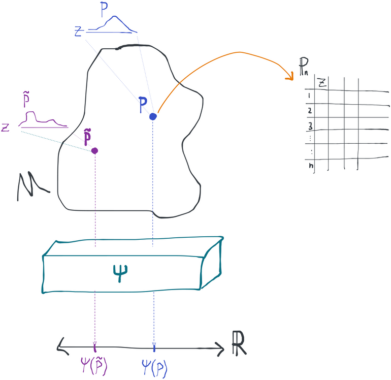
Here we see how the statistical model , estimand , and data are related.
We often talk about models that are "larger" or "smaller" than other models. By this we usually mean that one statistical model is a superset or subset of another, or that one includes a greater or lesser diversity of candidate distributions. If a model is "small", it necessarily imposes more assumptions because we are a-priori ruling out a larger number of distributions. For example, a model where we assume a variable to have a normal distribution is necessarily smaller (more restrictive) than one where, all else equal, we do not put any assumption on the distribution of that variable. On the other hand, "large" models require few assumptions because very little is ruled out a-priori: we instead rely more on the data to tell us which world we are most likely to be in.
Measure-Theoretic Probability and Notation
Here we take to be the probability measure of our observed data. It maps subsets of (the space takes values in) to numbers in and obeys certain rules like additivity over disjoint sets.
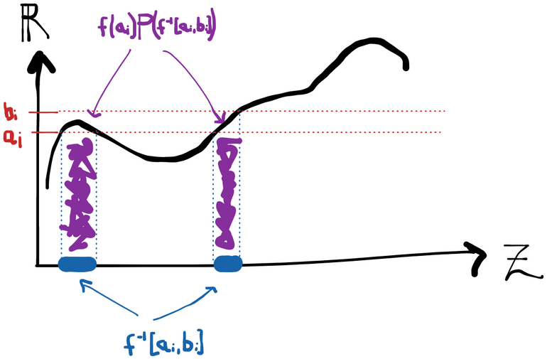
The (Lebesgue) integral of a function over a set with respect to a probability measure is written as , which is approximately the same as saying "break up into intervals and compute the finite sum ". Here means "the set of points in that end up going to the interval under . The role of here is to assign some notion of "length" or "weight" (or "probability"!) to the sets .
If we are integrating with respect to a measure that has some density (with respect to the "Lebesgue measure") then we can write . This latter form should look familiar from your introductory probability classes.
Obviously the value of the integral depends on what measure we integrate with respect to. We also call the integral of a function w.r.t. a probability measure the expectation of that function, denoted or even just . This latter is technically an abuse of notation since we're using both for the measure and as an operator that maps functions to numbers. However, it's a) very common and b) minimizes visual clutter, and c) makes it clear what underlying measure we're integrating with. If we use densities, we can write the expected value of some random variable with distribution as . Again this form should look familiar to you.
Parametric, semiparametric, and nonparametric models
A parametric model is one where each probability distribution can be uniquely described with a finite-dimensional set of parameters. For example, if we had a dataset where each takes scalar values, we might suppose that each observation is an identically distributed normal random variable. That's an assumption, of course, and it might not be realistic or good because that rules out a lot of other possible distributions. Nonetheless, it's one way we could define a statistical model.
Since is normal in this model, we can describe its full distribution with just a a mean and a standard deviation. Knowing only these two numbers tells us everything about the distribution. We say that this model is parametrized by these two numbers. An example of a slightly more complicated parametric model is a normal-linear model where each measurement in the data takes the form of a tuple and we assume . Now we have three parameters: the slope as well as the mean and the standard deviation of the normally-distributed random noise. Again, this implies a strict set of assumptions which may not be true: namely that the true relationship between and the conditional mean of is linear and that the conditional distribution of given is normal with a standard deviation that is fixed and doesn't depend on .
In general, having a parametric model means that we can write the density of the data as a function of some finite-dimensional vector of parameters (e.g. ). We might write the density like . Each value of in the domain implies one density in and each density in the model has one unique value of the parameters that characterizes it.
Parametric models are popular because they are easy to work with: finding the distribution most likely to have generated the data reduces to a finite-dimensional optimization problem in the model parameters. However, they are usually also completely artificial! Do you really believe that the "true" relationship between the dose you take of a drug and the toxicity is exactly a straight line? Any parametric model with a few parameters is necessarily a very "small" model that rules out the vast, vast majority of possibilities. Depending on the situation, basing statistical inference on a parametric model can give you completely meaningless inference: biased estimates and invalid confidence intervals and p-values. We'll have more to say about that later.
Semiparametric and nonparametric are both terms used to describe models that cannot be boiled down to a finite-dimensional set of parameters.
Empirical distributions
We use the symbol to denote an empirical distribution. This measure assigns mass at each of the points taken by the random variables . Mathematically, if we let be the measure that returns 1 if and 0 otherwise, then we can define . This is just the fraction of samples that happen to have fallen into the set .
What you have to remember about the empirical measure, though, is that it's random. In other words, evaluated at any fixed set is itself a random variable because the data themselves are taken to be random variables (with their own underlying distribution) in an inferential analysis.
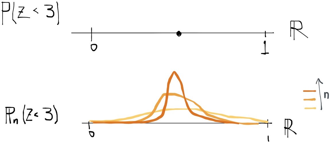
evaluated at some set is a random variable because the data that define it are random. evaluated on some set is a fixed number. As increases, the empirical distribution tends to concentrate around the value that takes.
Or you can think of as a random measure that takes values in the space of probability measures. In this case has a distribution over the model space itself. Once you fix a particular sample from , then the empirical distribution takes a single point value in . The empirical measure (for fixed ) is also one element of a sequence of random measures that in some sense gets closer and closer to .
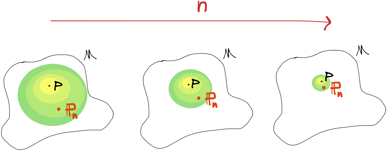
as a "density" over the model space with a typical realization shown. Note that this picture is just one possible example. In general, may take values that are actually outside of !
Any way you look at it, this is an example of a random "thing" that takes values in a set that isn't . Note that the empirical measure depends on the underlying distribution . So if we had a different underlying distribution, say , we might denote an empirical measure based on IID samples from as .
Independent and Identically Distributed
In this book, we will only consider statistical models where each observation is assumed to be independent and identically distributed (IID). In other words, we assume . Analytically, this is extremely helpful because we only need to describe the distribution of a single generic observation in order to describe the distribution of our whole dataset. Therefore when we talk about the statistical model, we're talking about the space of distributions of a single observation with the implication that the data distribution is .
This is an important assumption and limitation on the statistical model. A model where the data are IID is less generic (i.e. "smaller") than a model where we don't make that assumption. The reason we limit our focus is that the IID assumption is easily justifiable in many important problems. For example, in an observational study on cancer it's reasonable to presume that each subject is a sample from some eligible population (i.e. subjects are identically distributed) and that what happens to one subject doesn't affect what happens to another.
Nonetheless, there are many interesting and important problems where the IID assumption is untenable. For example, any large study of a highly infectious disease must take dependencies between subjects into account because any one person getting sick increases the chance that others get the disease. There is a large literature that deals with inference where observations cannot be considered independent. One useful trick is to clump observations into clusters which can themselves be treated as independent (e.g. cluster randomized trials), but this is not always possible. In general, however, it is important to understand the well-developed techniques for performing inference with IID data before you try to tackle more challenging problems that will require you to extend and build on these strategies.
Structural Equation Model
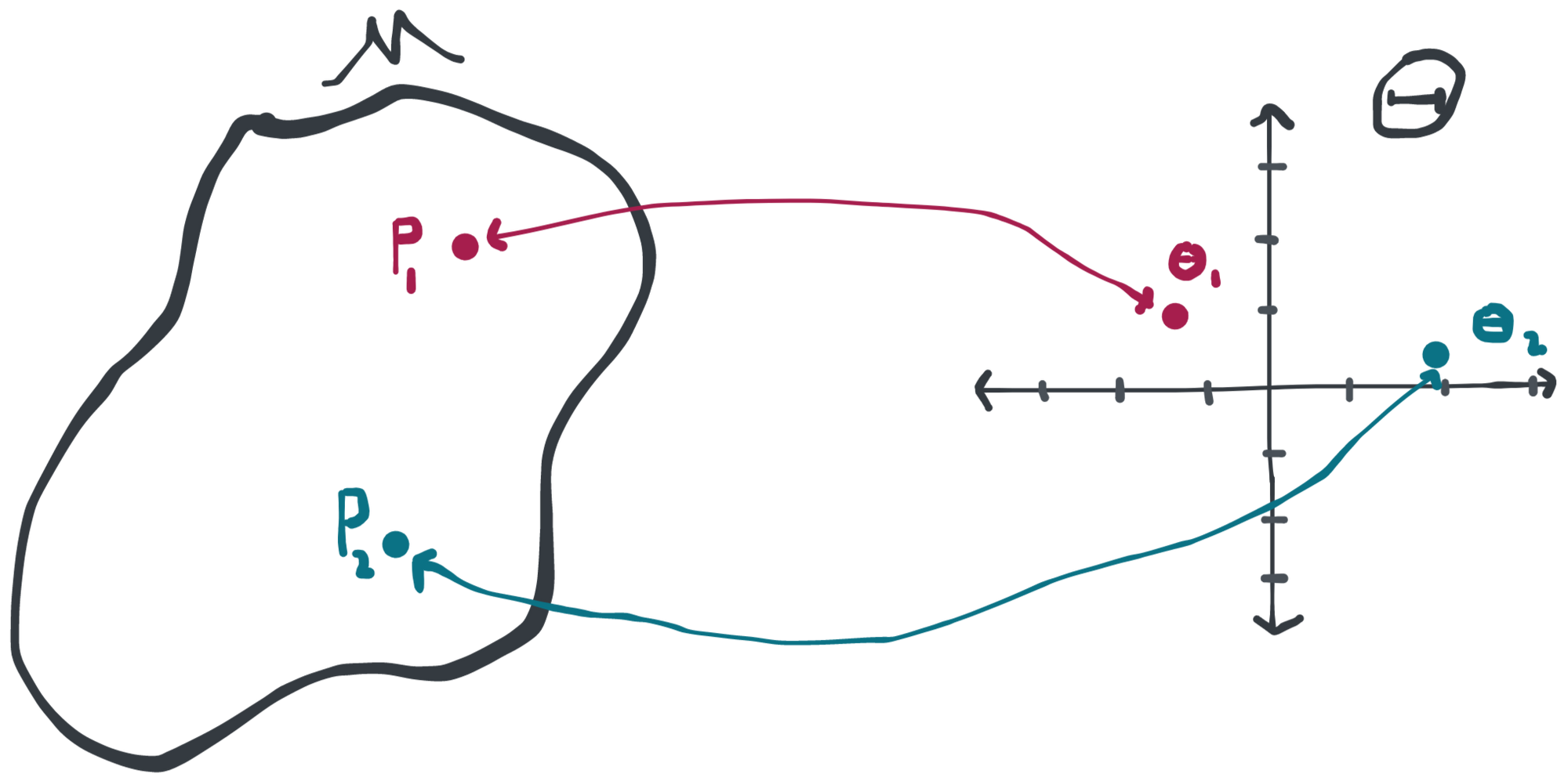
Each "point" in a statistical model is a probability distribution . As we move from one distribution to another, say , what exactly changes? How can we break up the model into pieces that allow us to reason more clearly about specific relationships?
A (nonparametric) structural equation model presents a solution to that problem. Let our observation be a vector of random variables . Recall that we can always factor an arbitrary joint distribution into a product of conditional distributions . It therefore suffices to describe each of the conditional distributions and the marginal distribution of (we can also, of course, reorder the indexing in any way that is convenient to minimize notational and analytical burden). That's the entire idea of a structural equation model. We can write any joint distribution of as:
Where are exogenous variables (basically a fancy word for "random" or "external" noise), none of which depend in any way on the observables , and are fixed (nonrandom) functions. We have therefore described the joint distribution of with the joint distribution of and the functions . Once these are specified, everything else follows. This way of specifying a distribution is what we call a structural equation model. You might also think of this as "parametrizing" the distribution with the random variables and the functions . The space of possible and define the statistical model, and any one choice of these identifies one particular data-generating process within the model.
The structural equation model is extremely generic because we can describe any distribution in this way. If we want to impose additional assumptions, it's easy to do so. For example, if we want to impose conditional independence between and given , we could specify , and . As another example, if we want to specify that has conditional mean given by and has normal conditional distributions with fixed variance , we can impose and . The possibilities are literally endless.
It can also be useful to draw a picture that specifies the conditional independence relations present in any given structural equation model. This kind of picture is often called a directed acyclic graph (DAG) or graphical model. To draw a DAG for a model, you first draw your random variables as nodes. For any given variable, you then look at its corresponding structural equation and draw an arrow into coming from any variable that appears on the right-hand side of the equation. Alternatively, you can have a DAG for a model and then translate it to a set of structural equations by following the reverse process. DAGs are necessarily a bit less expressive than the full algebraic structural equations, but there are many properties of complex joint distributions that can be more easily deduced by looking at a DAG than by reading through equations.
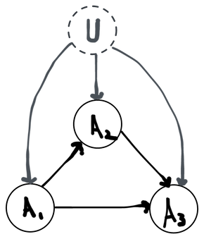
An example DAG for a model with three observed variables.
Example: Observational Study
To fix ideas we'll write up a structural equation model for a common use case: modeling an observational study. In our formal statistical model of an observational study, we imagine that for each subject we observe a vector of pre-treatment covariates (e.g. their age, sex, history of disease), an indicator of whether they received an active treatment () or not (), and a scalar that represents their outcome some time later (e.g. survival, score on a test, disease state). We'll factor the joint distribution as since this reflects the intuitive time ordering of the variables: the covariates are measured, then some treatment is given, and then finally the outcome is observed. The treatment that is received may depend stochastically on the covariates (e.g. sicker people may be more likely to receive treatment) and the outcome almost certainly depends stochastically on both the covariates and the treatment. We could also have ordered the factorization differently, but this factorization reflects our understanding of the world and gives a more intuitive meaning to each factor.
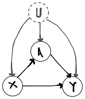
Notice that the only restriction we've placed on this model besides enumerating the variables is that the function return either a 0 or a 1 (enforcing the fact that the treatment is binary, which we know is the case). We've omitted since we can always write for arbitrary and so this is not an assumption. Thus for all intents and purposes we have not assumed anything that we don't already know is true. We don't know that the relationship between and is linear, or that the conditional distribution of is normal, etc. If we don't know those things to be true, why would we impose them on our statistical model?
Example: Simple Randomized Trial
Another example we can give is a simple randomized trial. A simple randomized trial is precisely the same as an observational study, except that that the experimenter has precise control over who gets the treatment and who doesn't. In other words, we know what is. In the simplest case, the experimenter assigns treatment to each subject on the basis of a coin flip. We can therefore write:
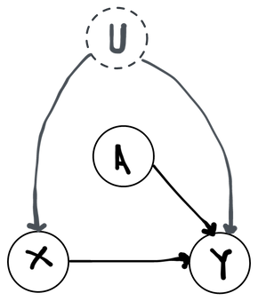
Notice that we've imposed the assumption that we know exactly what is (a coin flip) and what is (the identity). Controlling the distribution of in this way eliminates all incoming arrows. It therefore breaks all dependence between and : in a simple randomized trial the covariates have no role in what treatment someone gets. On the other hand, we still have not made any unfounded assumptions about because we don't know anything precise about how the covariates and treatment relate to the outcome. This is easy to see in the DAG, where it's now impossible to find a path from a common ancestor of both and that doesn't pass through (because has no ancestors!).
Estimand
Now that we've represented the space of possible worlds with a space of probability distributions, we have to represent our scientific question in the same terms. For example, let's say we're interested in what the "usual" temperature is on a day in San Francisco. A sensible way to formalize that would be to ask what the expected value is of a variable (representing temperature) with some given distribution: in other words, . Another question of interest might be: what is the average outcome (e.g. disease-free survival time) for a group of patients who were all exposed to a particular drug? In this case, we might represent each subject's outcome as a variable and their treatment status as (0 corresponding to no drug, 1 corresponding to drug) and the quantity of interest might be the conditional expectation .
We refer to the quantity of interest as the statistical estimand or statistical target parameter. Formally, an estimand is a mapping (function) from the statistical model to the domain of the parameter (usually the real numbers). In other words, each distribution in the model has its own (not necessarily unique) value of the estimand. This formalizes the fact that the answer to our scientific question is different in different "universes". We use the notation to denote the value of the estimand if the true data-generating distribution is . For example, if we had data and the estimand were the conditional mean of given , then we would have . Notice that the argument is what we're taking the expectation with respect to. We can write the expectation more explicitly either in the measure theoretic notation or if we have that the density of under is we'd write (as opposed to, e.g. for a different distribution ) . Either way, the point is to demonstrate why is itself the argument here: the estimand maps each distribution to whatever the "true" answer to our question would be if we were in the universe where our data were generated according to that distribution. That's why, if we knew , we wouldn't need any data at all to answer our question.
“Estimand” vs “target parameter”?
These two terms are completely synonymous in the context of modern causal inference.
In traditional (parametric) statistics, the statistical distributions could always be described with a finite number of parameters. These parameters (or simple functions of them) were always the objects of interest- i.e. the estimands. As statistics started moving into nonparametrics, the term “parameter” stuck around but acquired a new, generalized meaning as a generic attribute of a distribution. That was then formalized into the definition we have now, which is that a parameter is a mapping from the model space into, say, the real numbers. The point is that parameters are now defined in a way that divorces them from models, whereas it used to be that parameters really only made sense within their own models.
We think this shift is fundamental enough to constitute the use of a new term (”estimand”), especially since most people still carry around the more intuitive but limited perspective they learned in their first statistics class. Moreover, “estimand” makes it clear that this is the aspect of the distribution that you actually care about. “Parameter” is agnostic to the analyst, which is why you’ll see “target parameter” used to impose the required normativity.
I (Alejandro) like “estimand” because it’s shorter and makes for a cleaner mental break with the world of purely parametric statistics, but you’ll see “parameter” or “target parameter” used more frequently in the literature. Throughout this book we’ll use these terms interchangeably so that you get used to seeing both.
The term "estimand" is used in the literature to refer both to this mapping and sometimes also to the actual value that the mapping obtains at the truth (we also sometimes abuse notation and write to mean the value and not the function when it's obvious what is intended). If you like, you can think of the function as the "estimandor" and the value as the "estimand" (in analogy to an "estimator" and "estimate"). Just note that these aren't terms you'll find anywhere else. Either way, you should notice the parallel between an estimator and estimand(or): both are known functions that map distributions into real numbers (that's part of why it's nice to be able to write the data as the empirical distribution - we get a nice symmetry). Then there's also the parallel between estimate and estimand: both are real numbers, the former being a visible guess of the latter, which is unknown.
Inference
With these pieces in place we can now discuss inference, which is the process of assigning a formal notion of uncertainty to our estimate.
Imagine that we knew, with certainty, that our data were generated by taking random draws from a particular probability distribution . Since the estimator is a deterministic function of the data, we can directly compute the distribution of the estimate . It's important to understand that the estimate is itself a random variable, since the data are themselves random. The distribution of is called the sampling distribution of the estimate (or of the estimator). The sampling distribution is what we would get if we repeated our entire experiment under identical conditions (i.e. sampling observations from ) an infinite number of times and made a histogram of all the estimates we got each time. In reality, we only ever see a single realization of our experiment and a single realized estimate. We therefore need to use probability to imagine what would have happened if we repeated the experiment many, many times.
We never know , so the exact sampling distribution of our estimator is generally unknown. Most of the challenge of statistics is figuring out how to say something about the sampling distribution of an estimate despite not knowing everything about . Undoubtedly the most useful tool we have for this task is the central limit theorem, which says that the distribution of an average of IID variables starts looking more and more like a normal (specifically ) as the number of observations gets large. If our estimator takes the form of a sample average of some variable , or can be shown to behave like a sample average as the number of observations grows, then we can apply the central limit theorem to understand its sampling distribution. All we have to do is estimate and consistently.
Knowing the sampling distribution of our estimate is the key to quantifying the uncertainty we have in our estimate. While we could calculate any property of the sampling distribution, the two things we're usually interested are the bias and variance of our estimate.
Bias is the systematic error of our estimator: . This is the amount by which the center of mass of our sampling distribution for the estimate is shifted away from the true estimand . We generally look for estimators that are unbiased, or at a minimum that become unbiased as the number of observations increases (are asymptotically unbiased or consistent). The variance of our estimator is nothing other than . It is a measure of the "spread" of the estimate, or how much we'd expect our answer to vary just by random chance. Having an estimate of the sampling variance is key to constructing confidence intervals and p-values, which are the usual ways to quantify uncertainty.
One of the most important things to understand about inference is that the properties of any given estimator depend on the statistical model the estimator is used under. Under certain assumptions, an estimator might be shown to be unbiased and attain a particular sampling variance. But if those assumptions are violated, everything might be off the table. It is therefore of great interest to construct estimators that have nice properties under very general conditions so that our inference is not resting on unrealistic assumptions. In the next chapter I'll take you through a detailed example and you'll see what we mean.
Summary
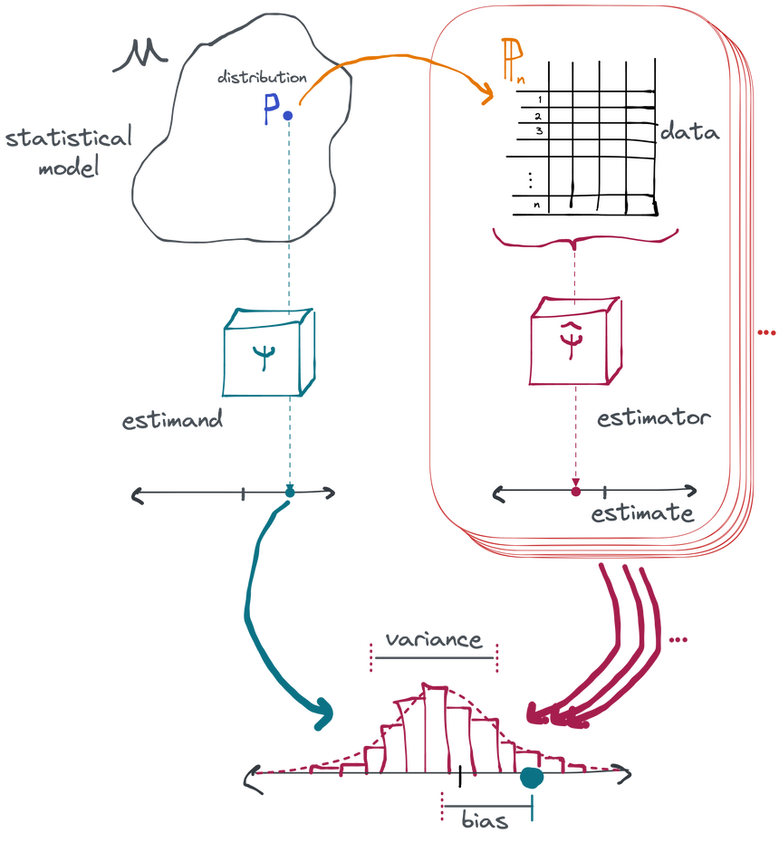
We can sum all of this up in one picture which neatly captures the pieces of an inferential analysis. The part inside the red rectangle is just a descriptive analysis. It's all you ever get to see in real life. But if you want to give your estimate a meaningful interpretation and measure of uncertainty, you need an inferential analysis. Inference requires you to imagine a space of possible distributions that could have generated your data (the model) and to identify a transformation that summarizes some characteristic of the distribution that you're interested in (the estimand). Finally, we derive how our estimate would vary across an infinite number of hypothetical repetitions of our whole experiment, drawing new data each time from the true distribution. From this we can establish, for example, that our estimate is right on average (has little or no bias) and is unlikely to vary more than a certain amount by random chance (has a particular variance). That's inference.