To fix the concepts I've introduced in the previous sections we're going to take a long, hard look at how linear regression might be used to estimate the effect of a treatment in an interventional study (either observational or randomized). First we'll motivate the definition of a treatment effect as an estimand. We'll then describe the usual maximum-likelihood version of linear regression as an estimator, which behaves well under the assumptions of the linear model. We'll then take this estimator outside of its "natural habitat" and show how it can be badly biased in generic observational studies. Lastly, we will show that this estimator is actually asymptotically unbiased in randomized trials, despite being motivated by a generally incorrect parametric model!
The point of this long exercise is to give you an idea of the danger of using "simple" methods without thinking critically about the relevant statistical model and estimand. It should also motivate our search for estimators that behave predictably and optimally across larger classes of problems.
Interventional Data and Average Treatment Effect
Throughout this section (and throughout most of this book) the estimand we'll be interested in is the (statistical) average treatment effect (ATE). Given the joint distribution of variables with the average treatment effect is defined as . Note that the outer expectation here is over the full marginal distribution of , not .
We usually call the outcome, the treatment, and the covariates. You can imagine, for example, a situation where represents a person's age, sex, and family history of disease prior to intervention, indicates whether that person received a new experimental treatment or a placebo treatment, and indicates their condition after the treatment. Throughout this book I'll refer to this kind of data structure (where we have covariates, treatment, and an outcome) as interventional data.
The conditional expectation function can thus be interpreted as the average outcome among those people with covariates who were treated with . The difference describes how the much average outcome increases for people with if they are given the treatment instead of . The ATE is just the average of this difference across the entire population (i.e. the average over the distribution of ).
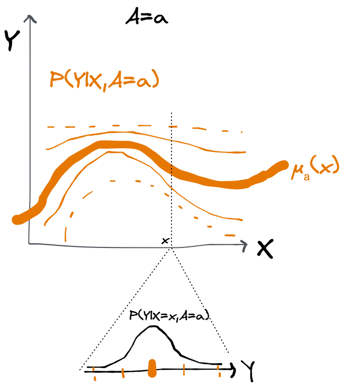
One useful way to think of the conditional distribution is as a set of distributions of indexed by . The conditional mean is what you get when you connect together the means of each of these with a line.
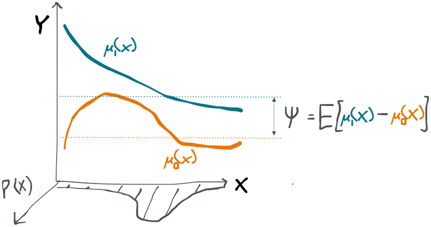
The average of the difference of the two conditional means is just their average difference weighted by the density of .
You can see why this quantity is of immense interest. If we can assure ourselves that the treatment can be changed independently of any other unobserved variables that would also affect the outcome, then the ATE tells us exactly how much better off we'd be prescribing the new treatment relative to the placebo in this population. It directly answers the question: "how well does this treatment work?" in terms of the population and outcome in question.
Strictly speaking, what we're talking about here is called the statistical ATE. That distinguishes it from something called the causal ATE which will be part of our investigations in the next chapter. We'll see that the two are the same as long as we can satisfy certain assumptions.
Remember that, as with all estimands, the ATE is a function of the joint distribution of the data. You can see that if you write things more explicitly as . Different distribution, possibly different ATE.
A Linear Regression Estimator
Now we've defined our general data structure and the estimand- all without having collected any real data at all. But let's say now we go and collect observations of . What do we do with that data in order to get an estimate of the ATE?
One very popular approach (but often unjustified, as we will see) is to use a linear regression estimator. The linear regression estimator is defined as the solution
Where we'll take to be our estimate of the true, unknown ATE . If we abbreviate and we can abbreviate this as . Taking a derivative with respect to and setting equal to zero gives the well-known analytical solution . The law of large numbers and limit arithmetic show that so as the number of samples we collect gets big, our estimates converge to this point that depends on what the data-generating distribution is, whatever it may be.
Unless you're already familiar with linear regression, this may look completely arbitrary. So why is this a common approach? Well, let's imagine that our statistical model consists only of parametric distributions that have the following form:
We'll call this statistical model (linear-normal). In other words, we assume that has some unspecified joint distribution, but that is linearly related to and plus some independent, normally distributed "error". Assuming linearity or gaussian errors is generally ridiculous in the real world, but let's go with it for now so we can motivate our estimator.
Since we have a parametric model, each distribution can be represented by the parameters of in addition to the nonparametrically unspecified . We can therefore construct the (log-)likelihood function of the parameters and maximize it to find the parameters representing the conditional distribution most likely to have generated the data (leaving nonparametrically unspecified). When you work out the algebra, the optimization problem comes out looking exactly like what we have above. Computationally, it can be solved analytically or by gradient descent, but that's not our concern here. This is where the linear regression estimator comes from. Moreover, the theory of maximum likelihood estimation ensures that has a sampling distribution that itself converges to a normal centered at the true value .
However, this argument only justifies why is a reasonable estimator of the parameter that exists in , but not why it is a reasonable estimator of the ATE ! The coefficient is just some number that describes the distributions within the linear-normal model. Without further justification, it has no inherent meaning.
Within the linear-normal model, however, it turns out that is in fact the same as the ATE. The proof is straightforward: taking the conditional expectation of shows , so . Taking the expectation over changes nothing. Thus, for the linear-normal model, we have that .
That justifies linear regression when we know that the true probability distribution is in . However, in reality, that is never the case. If , then doesn't even exist! The estimator can still be computed using arbitrary interventional data, but what does it mean? What can it mean? These are precisely the questions we will now turn to.
Linear Regression in an Observational Study
Let's keep the linear regression estimator, but change our statistical model to represent a generic observational study. In an observational study we follow a group of subjects who are assigned to their treatments by an unknown process and then we observe the outcomes later on. Based on that information alone, we can make no assumptions at all about the structure of the data-generating distribution:

The variables could be anything with the right domains (e.g. ) and could have any arbitrary joint distribution. The only exception is that here we've written as the sum of its conditional mean and the exogenous term , which forces to be mean-zero. This is just a notational convenience, though: we could have just as easily defined some to be arbitrary and then set . We call this statistical model (observational). Note that is much "bigger" than because it places fewer assumptions on what the joint distribution of is.
Our question now is: does the linear regression estimator still work to estimate the ATE in this larger statistical model? To answer this we need to look at what converges toward as we gather near-infinite amounts of data. We already claimed above that . This result was arrived at without any mention of a specific statistical model, so it is true generically. Therefore the question comes down to establishing
Where the dots are stuff we don't care about (in the linear model, they correspond to estimates of and ). If the central equality does not hold, then the estimate we get out of our linear regression estimator is likely to be near some value that isn't the ATE. If that were the case it would make no sense to use linear regression to try and estimate the ATE.
Unfortunately, that equality does not hold for in general. Obviously it holds inside , but the problem is that there are distributions outside of where things go wrong. We can give one such example. Presume the true distribution is specified by this probability mass function:
Here has three categories and is binary with a joint distribution such that they are more likely to be equal in absolute value (i.e. or or ) than not (i.e. ). The outcome is 1 if any only if and are equal in absolute value. You might imagine this is a scenario where is some kind of U-shaped indicator of the type of treatment someone would benefit from. If or then the best treatment is which results in the good outcome , but results in the bad outcome . On the other hand if then it is that gives the good outcome.
You can crank through the calculations (outlined in the toggle below) to find that in this scenario the ATE is . However, you can also calculate that for this distribution the limit of the linear regression coefficients is . Clearly so we conclude that linear regression is not a consistent estimator of the ATE in a general observational model! Even if we had infinite data, we would still get the wrong answer.
Calculations
Since everything is discrete, notice that we can compute expectations like using the values in the table above.
First let's calculate . We obtain which means .
Now we tackle using the same type of expansion to calculate each expectation in the terms below:
And multiplying these two together gives us the somewhat horrific .
Linear Regression in a Randomized Trial
Now let's work with a generic randomized trial. In a randomized trial we take a group of subjects, flip a coin to decide who gets what treatment, and then observe the outcomes later on. Based on that information alone, we can make no assumptions about the distribution of the covariates and how the affect the outcome (e.g. linearly), nor can we assume how the treatment factors into the outcome. What we can say for sure is that the treatment is independent of the measured covariates and of anything else that could possibly affect the outcome.

Here we are assured that and . We'll call this statistical model (randomized controlled trial). Any distribution of the form above is a special case of our other model , so we have that . The relationship with is also clear: there is some overlap (when is normal and is linear in and ) but there are also distributions in that aren't in because the latter imposes a very specific form on the distribution of . Therefore the two intersect but neither is a subset of the other.
We know the linear regression estimator is consistent in . We also know there are distributions in for which it is not. But are any of those distributions in ?
To figure this out all we need to do is calculate the linear regression limit under the assumption that and check that its last element is indeed the ATE .
We'll use one additional simplifying "assumption" here, which is that . This isn't actually an assumption because we can always center the observed covariates (call them ) and in the limit the empirical centering is equivalent to de-meaning. This is useful because (one of the terms in ) follows from the independence and . Moreover . Thus
Now we turn our attention to . The terms in are but since we're only interested in the last element of the vector and we see there is a 0 in the middle position of the last row of , it turns out that doesn't matter. Thus . Now we use the fact that and also that by the independence .
And thus by multiplication and subtraction we arrive at , which is exactly , the ATE. We have therefore proven that the linear regression coefficient is a consistent estimator of ATE in a randomized trial.
Conclusion
The takeaway message from all of this is that you need to think critically about the estimand, the estimator and the statistical model together to be able to claim that your method "works". Linear regression is widely used in the observational study literature because introductory statistics classes fail to emphasize that the maximum likelihood results require totally unrealistic assumptions (linearity, normal errors). In fact, many curricula fail to even mention that generally what is of interest is a parameter that is defined outside of a parametric model (e.g. the ATE vs. some fictitious coefficient ).
However, we also showed that, in some cases, linear regression still works to estimate the ATE despite the maximum likelihood assumptions not holding. This justifies the use of linear regression to estimate the ATE in randomized trials, which is also common practice. The point is, however, that this should be surprising rather than expected!
We haven't discussed this, but it turns out that the usual way of estimating the standard error (and thus confidence intervals and p-values) is not consistent outside of the linear-normal model, even in a randomized trial! That's why the sandwich estimator exists.
And what if we change the estimand? If is binary, we might consider using logistic regression to estimate a marginal odds ratio instead of the ATE. It's common practice to exponentiate the coefficient from a logistic regression fit and call it an odds ratio representing some effect of treatment. But this, too, is a problem, because even in the relatively safe haven of a randomized trial, one can show that this estimator is consistent for a weird estimand called the conditional odds ratio and not the marginal odds ratio that is most often of interest! Things are even worse in survival settings: the hazard ratio is essentially meaningless without the assumption of proportional hazards!
Use your brain!
The fact that inference is not taught from this perspective continues to create confusion in many fields. The big problem isn't about p-hacking, or frequentist vs. bayesian statistics, or this or that model. It's about not thinking clearly about the question and the assumptions.
Is it sometimes difficult to keep all of this in your head? Sure. But we promise that also gets much easier with practice! And it's certainly easier in the long run to understand the goal of your analysis and a framework in which to think than it is to try and memorize a flowchart of a hundred different methods that may all be wrong anyways. So think about the model, think about the estimand, and make sure your estimator makes sense in that context!