The naive plug-in estimate is fairly straightforward. We start with the data $\mathbb P_n$ (which is IID from $P$) and we use some kind of algorithm to come up with a guess for the probability distribution that generates it. We call that guess $\hat P$. We then evaluate our parameter at $\hat P$ to get the estimate. In other words, we define $\hat\psi(\mathbb P_n) = \psi(\hat P)$.

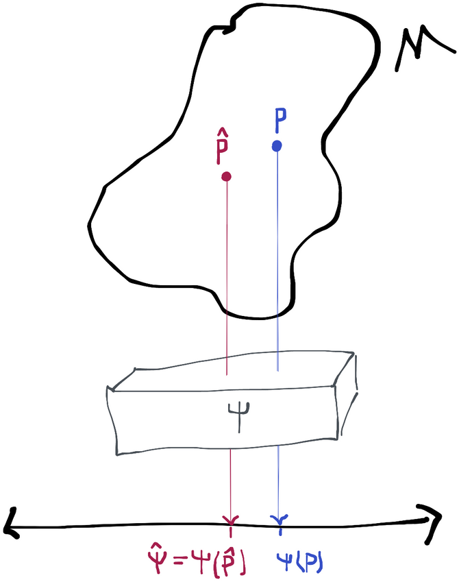
Recall that the efficient influence function (and influence functions in general) depend on what point $P$ we're at in the statistical model $\mathcal M$. We don't know $P$ so we don't know the efficient influence function for $P$, which is $\phi_P^\dagger$. However, we do know $\hat P$ so we can use the techniques from the previous chapter to find its influence function $\phi_{\hat P}^\dagger$, or $\hat \phi^\dagger$ for short.

For example, let's work with the $(Y,A,X)$ data structure that we'd find in an observational study and assume that our parameter of interest is the average treatment effect $\psi(P) = E_P[Y|A=1] - E_P[Y|A=0]$. As before, we'll notate $\mu_a(X) = E_P[Y|A=a,X]$ so we can also write the target parameter as $\psi(P) = P[\mu_1(X) -\mu_0(X)]$. For simplicity let's assume the outcome $Y$ is binary.

We need to use the data to come up with an estimate of the joint distribution. We can break that down by factoring $P(Y,A,X) = P(Y|A,X)P(A|X)P(X)$ and coming up with estimates for each factor. For example, maybe we use the empirical distribution of $X$ as our estimate $\mathbb P_n(X) = \hat P(X)$. We might also use a probabilistic classification algorithm (e.g. random forest) trained by regressing $A$ onto $X$ to estimate the probability of treatment $\hat\pi_a(X) = \hat P(A=a|X)$ and the same algorithm trained by regressing $Y$ onto $(A,X)$ to estimate the probability of an outcome $\hat\mu_a(X) = \hat P(Y=1|A=a,X)$.

Now we just need to apply the definition $\psi(P) = E_P[Y|A=1] - E_P[Y|A=0]$ but take the expectations with respect to our estimate $\hat P$ instead of the unknown $P$. Based on the estimates we defined above, and the definition of our parameter we get

Or, in words: take the sample average value of our estimate for the treatment outcome and subtract off the sample average value of our estimate for the control outcome. You might think of this as "imputing" the expected probability of the outcome under each treatment, for each subject in the study, and then averaging and taking the difference.

A naive plug-in estimator is nice because it's easy to understand and construct, but since we haven't said anything about what kind of algorithm we use to estimate $\hat P$ we can't ensure that the plug-in will behave nicely. As a stupid example, consider that we use some algorithm that completely ignores the data and always returns some fixed distribution $\hat P = P^\degree$. The plug-in estimate based on that distribution will always be the same number $\psi(P^\degree)$ so this estimator won't have a normal sampling distribution. Nor will it be centered at the true parameter unless we get lucky and $\psi(P) = \psi(P^\degree)$.

Our goal, therefore, is to come up with some "rules" that our estimator for $\hat P$ has to follow in order to make the plug-in estimator asymptotically linear with the efficient influence function:

From here on I'm going to use $\hat\psi$ and $\psi$ interchangeably with $\psi(\hat P)$ and $\psi(P)$ to keep things uncluttered when necessary. I'll also omit the dagger ($\dagger$) as a superscript of the efficient influence function, since from here on out we won't be talking about any influence functions that aren't efficient.

We want to get an idea of the magnitude of the estimation error $\hat\psi - \psi$. We actually have a pretty nice way to do this if we construct a path from $\hat P$ to $P$ and then use the pathwise derivative along this path, exploiting the fact that we know how to express the pathwise derivative at 0 as the covariance between the path's direction (the score $h$) and the canonical gradient of the parameter $\psi$ at $P$ (which is the efficient influence function $\phi_P$). To wit:

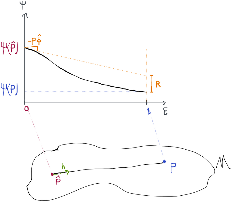
In this case $\Delta\epsilon = 1 - 0$. The equality in the last line is because $E_{\hat P}[\hat\phi h] = \int \hat\phi h d\hat P = \int \hat\phi dP = P\hat\phi$ by the definition of the score $h$ along a path from $\hat P$ to $P$ and the change-of-variables formula.

This is called the von Mises expansion of our estimate, which is a lot like the first-order Taylor expansion you may have seen in calculus. The idea is to use a derivative at a point and the value at that point to estimate the value of the function at a nearby point. It is an approximation, however. Because we let $\Delta \epsilon = 1$ be some finite value, the linear approximation won't be perfectly accurate. We'll call the approximation error $R$, so we have that $\hat\psi-\psi = R - P\hat\phi$.

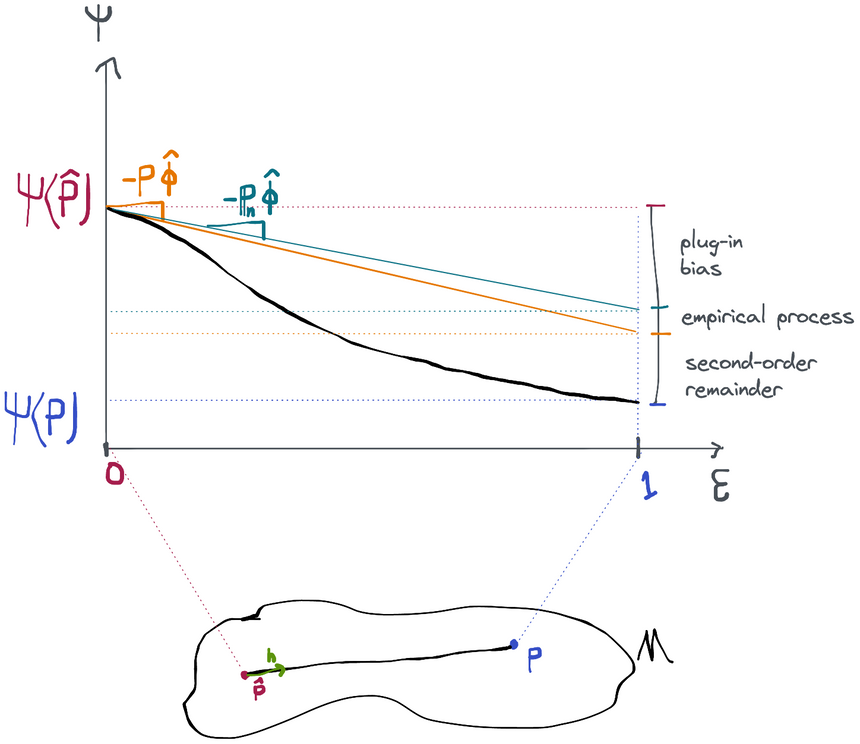
This gets us a little closer to where we want to go. Starting from here, we can add and subtract $P\phi$, $\mathbb P_n\phi$, and $\mathbb P_n \hat\phi$ to the right-hand side and rearrange terms to get

Now we're good. Comparing this to the characterization of an efficient estimator $[\hat\psi - \psi] = \mathbb P_n\phi + o_P\left(\frac{1}{\sqrt n}\right)$ we see that for our estimator to be efficient, the sum of the three terms after the "efficient central limit theorem (CLT) term" $\mathbb P_n \phi$ needs to be $o_P(1/\sqrt n)$ to make the two characterizations match up. This will be the case if each of the three terms is $o_P(1/\sqrt n)$, so that's what we need to show. We'll give each of these terms names and get to know them more intimately one-by-one:

The term $-\mathbb P_n\hat\phi$ is known as the plug-in bias term because, in general, it's not possible to show that it goes to zero at all for a generic plug-in estimate $\hat P$. If it doesn't go to zero, that makes our parameter estimate $\hat\psi = \psi(\hat P)$ biased, which is not at all what we want.

The three different strategies for building efficient estimators that we're going to learn about differ only in the way that they ensure this term is eliminated. All of these methods eliminate the plug-in bias exactly without needing to make any additional assumptions about the initial plug-in estimate $\hat P$. We'll talk a lot more about that later.

The term $(\mathbb P_n - P)(\hat\phi-\phi)$ is known as the empirical process term because there is an entire field called empirical process theory that studies things that look exactly like $\sqrt n (\mathbb P_n - P)f$. These creatures are called empirical processes because they are special kind of stochastic processes based on the empirical distribution $\mathbb P_n$.

We'll see there are two ways we can make sure this term is $o_P(1/\sqrt n)$: sample splitting and Donsker conditions. We'll discuss what these are shortly but for both of them we will need to assume that $||\hat\phi(Z) -\phi(Z)||^2 \overset{P}{\to} 0$ where the norm is the $\mathcal L_2$ norm $||f||^2 = \int f^2 dP$. This is nothing but saying that the true mean-squared error of $\hat\phi$, viewed as a prediction of $\phi$, goes to zero. Note $\hat\phi$ is itself a random function (because $\hat\phi$ comes from $\hat P$, which comes from the random data). In this notation we are not averaging over the variability of $\hat\phi$ itself when we take the norm so therefore $||\hat\phi(Z) -\phi(Z)||^2$ is itself a random variable and the convergence is in probability. We call this condition $\mathcal L_2$-consistency (of the estimated influence function).

This is the first restriction that we need to impose on the plug-in estimate $\hat P$ to ensure we get an efficient estimator of $\psi$. In fact, without this assumption, not only could our estimator be inefficient, it might not even be asymptotically normal.

You may wonder whether this $\mathcal L_2$-consistency condition is reasonable to assume. The truth is that in most cases it's very easy to satisfy! In other words, it's not even an assumption, it's just a required condition that we have to make sure we meet.

For example, when estimating the ATE in an observational study, we know the influence function depends on $\hat P$ through the functions $\hat\pi$ and $\hat\mu_a$. If you do a little bit of "limit algebra" with tools like Slutsky's theorem and the continuous mapping theorem you can quickly show that all that is needed for $\mathcal L_2$-consistency of $\hat\phi$ is $\mathcal L_2$-consistency of $\hat\mu_a$ and $\hat\pi_a$ (and a uniform bound keeping $\hat\pi_a$ away from 0, but a) since we already assume this for $\pi_a$ for identification, this is very reasonable and b) this is easy to enforce by truncating the output of the estimate). Why is that good? Well, a large number of commonly used machine learning algorithms have been shown to be nonparametrically $\mathcal L_2$-consistent (e.g. highly-adaptive lasso, nearest neighbors, deep learning, boosting, and random forests). So if we estimate $\hat\mu_a$ and $\hat\pi_a$ using any of those machine learning algorithms, or any cross-validated ensemble of them, then we know we satisfy the $\mathcal L_2$-consistency condition and we have nothing to worry about from the empirical process term: it will go to zero quickly in large samples as long as we also meet one of the two following criteria.

The simplest way to make sure this term goes away is to use sample splitting (also called cross-fitting or cross-estimation). The idea is to estimate all the parts of $P$ that go into the influence function using one sample and then to evaluate the estimator using another sample.

For example, when estimating the ATE in an observational study, we know the influence function depends on $\hat P$ through the functions $\hat\pi$ and $\hat\mu_a$. If we were using sample splitting, we'd split our sample $(Y,A,X)_{1,\dots n}$ in two, let's say into two datasets (1) $(Y,A,X)_{1,\dots m}$ and (2)$(Y,A,X)_{m,\dots n}$. The first of these we will use to estimate $\hat\pi_a$ and $\hat\mu_a$, which we then take as fixed. We then evaluate the plug-in estimate using only the second sample: $\hat\psi^{(2)} = \frac{1}{n-m} \sum_{i=m}^n \hat\mu_1(X_i) - \hat\mu_0(X_i)$ (in this case we don't need $\hat \pi_a$ for the plug-in estimate). We can then reverse the roles of the two datasets to get $\hat\psi^{(1)}$ and obtain our final estimate as the average of $\hat\psi^{(1)}$ and $\hat\psi^{(2)}$.

If this sounds sort of like cross-validation to you, that's exactly right. It's the same idea and the same procedure. The only difference is that we're using the "validation sample" to get an estimate of the parameter $\psi$ instead of specifically using the validation sample to estimate the MSE of some prediction function.

Just as we do in cross-validation, this process can be extended to multiple ($K$) splits instead of just two. When we do this we use notation like $\hat\phi^{(-k)}$ or $\hat\mu^{(-k)}_a$ to denote the influence function and its components estimated using the all the data except for the $k$th fold and we use $\mathcal I_k$ to denote the set of indices $i$ that are included in the $k$th fold.

A relatively brief proof shows that if we use sample splitting and we assume the $\mathcal L_2$-consistency condition on $\hat \phi$, then the empirical process term is indeed $o_P(1/\sqrt n)$ as desired. This is remarkable because, as we've already discussed, in most cases it's pretty easy to prove $\mathcal L_2$-consistency for $\hat \phi$. So all we need to do to ensure that the empirical process term goes away is to use sample splitting, something we can implement with a simple for loop in code.

The only downside of using sample-splitting to control the empirical process term is that you might be afraid of some finite-sample bias that comes from effectively using less data. This should never be an issue in large samples, but may be of concern in small studies.

The alternative to using sample splitting is to assume that our estimate of the influence function $\hat\phi$ falls into something called a Donsker class. A Donsker class is just a family of functions that are not "too complicated". There are many examples, for instance all functions that are of bounded variation (think: bounded total "elevation gain" + "elevation loss" for a function of 1 variable) form a Donsker class. This example in particular is a very big class of functions, especially for a fixed bound that is large.

If $\hat\phi$ is Donsker and $\mathcal L_2$-consistent, it follows immediately from an important result in empirical process theory (lemma 19.24 in vdV98) that $(\mathbb P_n - P)(\hat\phi-\phi) = o_P(1/\sqrt n)$. The proof of that requires more asymptotic statistics that I'd like to assume you already know, but if you're curious (and comfortable with the material in chapter 2 of vdV98), then by all means go ahead and read chapter 19 of vdV98!

So how do we make sure we satisfy the Donsker condition (i.e. make sure $\hat\phi$ is in a Donsker class)? Well, thankfully there are theorems that show that Donsker properties are preserved through most algebraic operations (again, see vdV98 ch. 19). The upshot of that is that if we can estimate the components of $\hat P$ that we need for $\hat\phi$ in a way that guarantees they fall in Donsker classes, then $\hat\phi$ will be Donsker. In our observational study ATE example, that means that whatever machine learning algorithms we use to learn the functions $\hat\mu_a$ and $\hat\pi_a$ need to always return functions that are in a known Donsker class if we want $\hat\phi$ to be Donsker.

There are two major problems with this. Firstly, the vast majority of machine learning algorithms are not guaranteed to return learned functions that are in some Donsker class (though some, like highly-adaptive lasso, are). Secondly, for $\mathcal L_2$-consistency to hold at the same time as the Donsker condition, we must assume that the true influence function also falls into some Donsker class (technically the same one as our estimates, but since unions of Donsker classes are Donsker we can just join the two). Donsker classes are very often quite big so this isn't that crazy of an assumption to make. Nonetheless it's something to be aware of.

Overall, Donsker conditions are a less robust way of controlling the empirical process term relative to sample splitting because they impose stricter requirements on the algorithms you can use to estimate the components of $\hat P$ and also because they imply a restriction on the model space $\mathcal M$. However, in small data settings these may be reasonable costs to pay to ensure asymptotically efficient inference without having to do sample splitting.

The term $R = [\hat\psi -\psi] + P\hat\phi$ is known as the second-order remainder because, like the empirical process term, it can usually be shown to disappear at a "second-order" rate like $o_p(1/\sqrt n)$ or better under certain conditions. The difference is that these conditions are often specific to the exact parameter and model we're working with, unlike the empirical process term which we've seen can be bounded in a very general way. Therefore the most general condition we can impose on $\hat P$ is that the estimate behaves in a way such that $R=o_P(n^{-1/2})$.

Depending on the problem, this may require us to be able to estimate regression functions (like $\mu_a$ and $\pi_a$ in our running example) at fast rates. This is a strong condition that we'll say more about below.

For example, consider again the ATE in an observational study, or, to simplify things, just the conditional mean $\psi_a = E[Y|A=a] = E[\mu_a(X)]$. We can now exactly compute the second-order remainder using the expression for the influence function we previously derived:

The notation doesn't make it terribly clear, but the expectations and norms here are with respect to $(Y,A,X)$ alone- we're not averaging over the randomness in the estimation of $\hat\mu_a$ or $\hat\pi_a$ (remember these come from $\hat P$, which is something we estimated from the data). One way to think of this is to imagine that we've used a separate sample to estimate $\hat\mu_a$ and $\hat\pi_a$ and these expectations are conditional on the (independent) data in that sample. As a consequence, $R$ is indeed a random variable.

Given the final expression we've arrived at, a set of sufficient conditions for $R=o_P(1/\sqrt n)$ is that $\| \pi_a(X) - \hat\pi_a(X)\| = o_P(n^{-1/4})$ and $\| \mu_a(X) - \hat\mu_a(X)\| = o_P(n^{-1/4})$. This is because $o_P(n^{-1/4}) o_P(n^{-1/4}) = o_P(n^{-1/2})$. We could also require that one of these goes faster and the other slower, as long as the product of the rates is $n^{-1/2}$.

Asking for an $o_P(n^{-1/4})$ rate on the estimation of the functions $\hat\mu_a$ and $\hat\pi_a$ is much stronger than the consistency we required to control the empirical process term (that's just an $o_P(1)$ requirement). For the latter, we just need that those functions go to their true values in the limit as we get more and more training data. For the former, we need that limiting behavior to happen fast enough. If the rates are too slow, we can't guarantee that the $R$ term gets small fast enough for the efficient central limit term to dominate in large samples. As a result, our estimator might not even have a normal sampling distribution, which would crush any chance we have at performing inference.

Without putting unrealistic smoothness conditions on the true functions $\mu_a$ and $\pi_a$, it is very, very difficult to attain the required $o_P(n^{-1/4})$ rate, even with a machine learning algorithm. In fact, there are some general theorems that show that attaining such a rate is impossible if we assume general high-dimensional function spaces without such smoothness conditions. This is called the curse of dimensionality.

The curse of dimensionality made efficient inference in observational studies difficult if not impossible in the general nonparametric model. The strategy in the past was to use a cross-validated ensemble of machine learning methods and pray that the true function was smooth or low-dimensional enough that one of these methods actually could attain the $o_P(n^{-1/4})$ rate or better. Cross-validation is known to asymptotically select the best learner, which justifies this strategy as long as prayers are granted.

The highly-adaptive lasso (HAL) is a recent method for supervised learning that effectively solves this problem. Under non-restrictive assumptions, HAL can attain the $o_P(n^{-1/4})$ rate (better, actually!). This is astounding. HAL still requires an assumption to be made on the regression function of interest (thus restricting the model space) but this assumption is much more believable than asking for low-dimensionality or smoothness. Specifically, HAL asks that the true regression function (e.g. $\mu_a$) is right-continuous with left limits (cadlag) with bounded variation norm. This norm can be arbitrarily large, as long as it is finite. But this is barely an assumption at all because it's difficult to imagine a real world scenario with a regression function that isn't cadlag with bounded variation norm. The genius of HAL and the trick to how it "breaks" the curse of dimensionality is that it places no restrictions on the local behavior the regression function (e.g. how wiggly/smooth it is) but instead restricts the global behavior (how much it can go up and down in total).

In the observational study example we saw that the second-order remained could be controlled if the product of two rates is $o_P(n^{-1/2})$. This happens in several other estimation problems so there is a general name for the phenomenon. When the second-order remainder takes such a form, we say that the estimation problem is doubly robust.

The reason this term is appropriate is because we have two chances to completely cancel out the second order remainder term. For instance, consider the ATE observational study example, but now presume that $\pi_a$ is known (i.e. we're in an RCT). Then $\| \pi_a(X) - \hat\pi_a(X) \| = 0$ so the whole $R$ term is exactly 0. The same thing happens if we know $\mu_a$.

Double robustness is a property of the estimation problem, not of any particular estimator. Some estimators that use both $\hat\pi_a$ and $\hat\mu_a$ (or equivalents for the estimation problem in question) are sometimes called "doubly robust", but it's most accurate to say that these estimators exploit double robustness to attain efficiency and asymptotic normality under certain conditions (e.g. $o_p(n^{-1/4})$ rates on the regression estimates). Moreover there are estimation problems that may have triple, quadruple, etc. robustness, or only single-robustness (i.e. only a single function needs to be estimated), etc.

Double robustness was historically more important than it is today because parametric models were used more often to estimate nuisance components. It's rarely if ever the case that a parametric model can capture the truth, but at least if you have two (or more) chances to be right then there's a little more hope. On the other hand, double robustness says nothing about what happens when both models are wrong, even if one or the other is still "close" enough in some sense. Since that's more realistically the case with parametric models, some have argued that the entire premise is somewhat meaningless. Either way, it's rarely justifiable to not to leverage modern, flexible estimators like HAL in current practice, so assuming consistency of nuisance components is no longer a matter of hope. This makes the entire question of double robustness more of a moot point than it has ever been.

By analyzing the naive plug-in estimator, we managed to come to the following decomposition of estimation error that shows us exactly what conditions must be satisfied in order for our plug-in to be efficient.

Specifically, we need the following three terms to be $o_P(n^{-1/2})$:

And we came up with the following conditions to ensure that these terms do indeed go away:

Effectively, we have found reliable ways to control both the empirical process and second-order remainder terms, as long as a) the components of our plug-in $\hat P$ are modeled with powerful machine learning techniques that converge quickly to the truth as data are added and b) we use sample splitting or algorithms that guarantee their estimates are not too flexible.

The only thing that we're missing, therefore, are conditions or methods that control the plug-in bias. There are three ways that have been proposed over the years to handle this and that's exactly what we're going to discuss in the subsequent sections. Once this is handled, we've got an estimator that has the efficient influence function and therefore attains the minimum possible asymptotic variance!

The conditions required for control of the empirical process and 2nd order remainder terms are all totally attainable in practice, meaning that we can build efficient estimators for most estimation problems without making any scientifically meaningful statistical assumptions. Remember, however, that we usually do need scientifically meaningful causal assumptions in order to link our statistical parameter to a causal parameter of interest! These are separate, though, and apply uniformly regardless of how we choose to estimate the statistical parameter.