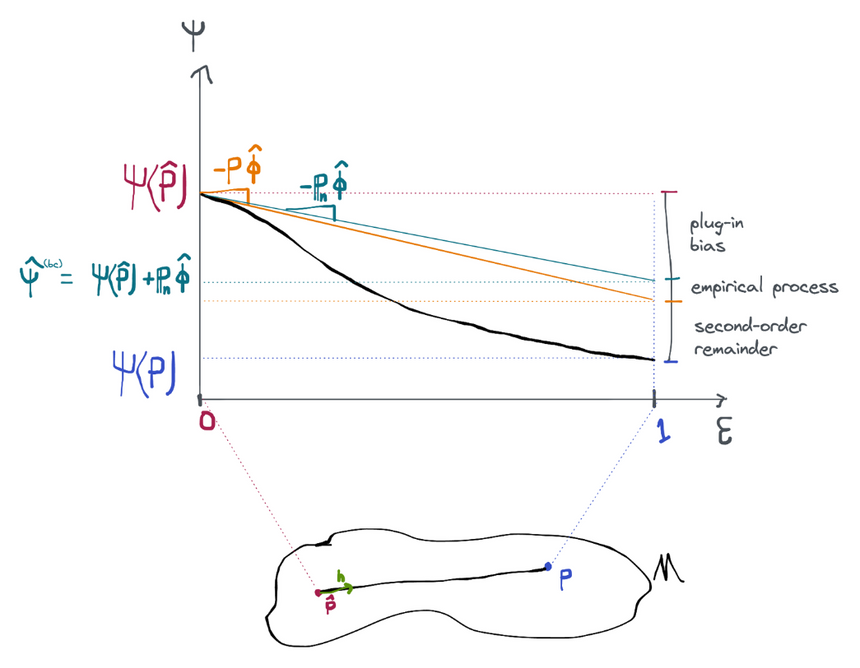
In the previous section we established that the naive plug-in estimator would be efficient if we could figure out a way to control the plug-in bias term (assuming the required components of were estimated with powerful enough machine learning methods so that the empirical process and second-order remainder terms go away).
One way to get rid of this term is to just calculate it and add it back in to the estimator! So instead of the pure plug-in estimator we use ("bc" standing for "bias-corrected"). This is possible because the bias term can be computed: is just a sample average and is just the efficient influence function for the estimated distribution , which is known by construction. We call this the bias-corrected efficient estimator.
Example: ATE in Observational Study
Recall that our plug-in estimate of the conditional mean is given by
where is an estimate of the true conditional mean that we get by running some kind of machine learning regression algorithm on the data. We also estimate using similar techniques. Using the expression we derived for the canonical gradient of the ATE in the nonparametric model, we have that
Taking the sum gives the bias-corrected plug-in estimate
From which we can get an efficient ATE estimate . This particular estimator is sometimes referred to as AIPW, or augmented inverse propensity weighting. You may also see it referred to as the "doubly robust" estimator, although, as we've discussed, this doesn't really tell the full story.
AIPW with sample splitting
If we use sample splitting to ensure the disappearance of the empirical process term, we might also write the above very explicitly as
where and are the estimates trained on the folds of data that exclude (at a minimum) observation .
Efficiency
The proof that this estimator is efficient is simple. Starting from the expansion of the naive plug in:
Done! This shows that has the efficient influence function assuming that the initial plug-in gives us fast-enough rates of convergence for the nuisance parameter required to get rates on the empirical process and 2nd-order remainder terms. We have already discussed how those rates are attainable if we use, for example, sample splitting and flexible machine learning estimators to construct our plug-in.
One intuitive explanation for why this estimator works is that it is effectively approximating a single "gradient descent" step along the path from to in order to get a bit closer to . The true derivative at is actually , but since we don't know what is we do our best to approximate that derivative using the sample average . Because of this interpretation as a single step of gradient descent, bias-corrected estimators are often called "one-step" estimators.
Discussion
Bias-correction is a general purpose strategy to build efficient estimators, assuming we can control the empirical process and second order remainder terms using the plug-in arguments from the previous section. The obvious benefit of this method is that it is super simple to implement: use a sensible plug-in estimate that goes to the truth fast enough, then add on the sample average of the efficient influence function at that plug-in estimate.
A potential downside of this estimator is that in finite samples it can produce values that are outside of the natural range of the parameter. For example, consider estimating the ATE in a situation where the outcome is binary. In that case, the true ATE must fall in the interval . However, in finite samples the bias-corrected plug in estimator given above can produce estimates that are less than 0 or greater than 1! This is very unlikely to occur in large-enough samples, but it can happen, especially if the outcome is rare. This is an unsettling property.
Another problem is that bias-corrected estimates are sometimes unstable in finite samples. In the ATE example, you can see that the estimated influence function includes division by the function . If this value is near 0, this can amplify smaller errors in the outcome regression model and make the entire estimator very unstable. This is a well-known phenomenon and in practice people use a variety of heuristics like weight stabilization or truncation (at relatively large values) in order to avoid these issues. Using these heuristics implicitly establishes some assumptions on the statistical model, which is unfortunate. They also give an ad-hoc feel to the estimator, which undermines the strong theoretical justification.
Nonetheless, bias-correction is a well-grounded technique that is often used to create asymptotically efficient estimators for a given parameter in a specified statistical model. In large enough samples, the bias-corrected plug-in is provably optimal.
History
If you're interested in the lineage of this strategy or where to find more details, Mark van der Laan gave a great summary in one of his blog posts:
Historically, the first efficient estimator was the so called one-step estimator using sample splitting (the work of Levin, Pfanzagl, and Klaassen circa 1970-1980, see references in the book by Bickel, Klaassen, Ritove, and Wellner). For example, Klaassen (1986) showed that the one-step estimator using sample splitting is efficient under minimal conditions. The one-step estimator (and its non-sample splitting version) is the efficient estimator presented in the comprehensive book on efficient estimation in semiparametric models (Efficient and Adaptive Estimation for Semiparametric Models) by Bickel, Klaassen, Ritov, and Wellner (1997). This one-step estimator is defined as a plug-in initial estimator of the target parameter, plus the empirical mean of the EIC at this same initial estimator. The sample splitting variant of this estimator is defined as the average across a number of sample splits in training and validation sample (say, V-fold), of the initial plug-in estimator based on a training sample plus the empirical mean over the validation sample of the EIC at this same initial plug-in estimator (fitted on the training sample). A little later (circa 1980 and onward), as empirical process theory emerged as a field, the sample splitting based one-step estimator was often replaced by the “regular” (non-sample slitting) one-step estimator that relied on the Donsker class condition (i.e., the sample splitting will come at a small price if the Donsker class condition nicely holds, but one should make sure that the initial estimator is not overfitted).