As we saw in the last section, identification is the process of mathematically tying a statistical estimand to the causal estimand of interest. Since we can observe data from the statistical distribution, we can infer the value of the statistical estimand. The identification result takes us the final mile and makes that inference causal.
There are cases, however, where we just can’t get the identification result we need to get a causal interpretation. For example, let’s say we have an observational study and we know we’ve missed an important confounder (e.g. some socioeconomic indicator). We also don’t have any special structure we can exploit to identify a different estimand, or perhaps we’re really only interested in the ATE (e.g.). In that case, we can still proceed with our analysis and get an estimate of the statistical estimand , but we can’t say that that the statistical estimand represents our causal estimand .
The difference between these two, i.e. , is what we call the causal gap. The causal gap isn’t something you can ever observe. You don’t know the true values of the causal or even statistical estimands. But it’s a concept you should keep in the back of your head when you’re estimating the statistical estimand. Ask yourself: even if I had infinite data, how far off might I be from the true answer to my causal question? Do I really believe in a set of identifying assumptions that would give a causal interpretation to this estimate?
Thinking there is a causal gap isn’t the end of the world though. You can still often say something useful without identifying your causal estimand. For one, maybe it’s already good to know whether or not there appears to be a statistical association between the outcome and treatment- by itself that could be grounds for further, more careful investigation. There are also pre- and post-hoc methods you can use to interrogate and communicate the causal gap: that’s what this section is about.
Lastly, you should also remember that the causal gap is just one part of the total estimation error:
Even if your estimand is identified, you still have to estimate it well in practice to get small statistical error. The statistical error is itself decomposable into statistical bias and statistical variance components. So if you use an inconsistent estimator (e.g. linear regression in an observational study), you get statistical bias on top of the bias from the causal gap. And if you have a small dataset, your statistical variance may contribute much more to total error than the causal gap.
That said, the statistical error is exactly what we try to control with statistical tools. We use consistent estimators so the statistical bias is (at least asymptotically) zero. We use confidence intervals and p-values to quantify the amount of statistical variance, which we keep small by using efficient estimators (the subject of the next two chapters). Point being: we already have tools to control, interrogate, and communicate statistical error. What we need are the equivalent tools to for the causal gap.
Partial Identification
We actually already have an extremely powerful tool to control the causal gap: an identification proof! If we have identification, the causal gap is eliminated completely. But in this section we’re interested in cases where we can’t prove identification of our causal estimand. It turns out identification proofs can still help us sometimes- we just have to shift the goalposts a little bit.
Instead of finding a statistical estimand that is always equal to the causal estimand, sometimes we can find one that is always greater than or equal to the causal estimand (and typically another that is always less than or equal). To make the discussion simpler, let’s assume that we know so we only care about an upper bound. Then, formally, what we’re looking for is a statistical estimand such that for all .
We haven’t eliminated the causal gap, but the point of this is that we have bounded it. For any hypothetical statistical estimand that we pick such that , we know we get a bounded causal gap: .
The process of identifying is called partial identification. This is in contrast to point identification, which is what we’ve been discussing so far. In partial identification, we’re formally estimating a set that contains the true causal parameter, not the exact value of the causal parameter (which would be impossible without more assumptions).
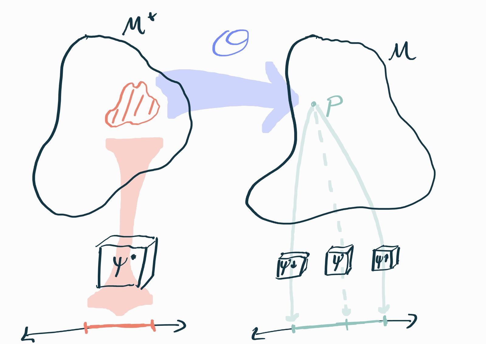
Here there are a number of causal distributions that all map to the same statistical distribution, making causal estimand unidentifiable by the statistical parameter . In effect, many values of are equally compatible with full knowledge of . However, the statistical estimands and can still give us provably accurate bounds on .
Once we find a bounding statistical estimand we can use data to generate an estimate of it with our usual estimation toolkit. We then have a bound where the upper boundary holds with some probability that we can try and quantify with confidence intervals or p-values on .
Example: Deterministic Treatment
Consider an observational study with a binary outcome where treatment was deterministically assigned on the basis of a single binary covariate (i.e. ). Our target causal parameter is , the outcome rate if we were to treat everyone in the population.
The problem is that we have absolutely no way of knowing what happens when we treat people with because we have nobody like that in our study sample. Formally, this is a violation of the positivity assumption: . Thus we cannot identify .
We can however, identify an upper bound! Consider the structural equations:
Then, by iterated expectation,
The constant we can estimate by the sample proportion with (call it ). Similarly, we can identify without difficulty and estimate that as the outcome rate in our sample among those people with and (call it ). The problem is the remaining term, , which we cannot identify due to the positivity violation (the conditioning event has zero probability).
What we do know is that , since this number is a probability. From this we can derive bounds on
These two bounds are identified and we can estimate them by plugging in and . If the point estimates for these are, say 0.2 and 0.5 and we have enough data that their variances are negligible, then the conclusion would be . This example is very simple and the bound we get isn’t particularly tight, but the point is to help you understand the mechanics of partial identification.
More examples and a more thorough explanation are given in Tamer 2010. Partial identification is a rich field in and of itself- this section is just a starting point for you to understand the general ideas.
Sensitivity Analyses
Partial identification is a “prospective” way of dealing with an identification problem in the sense that we change what we set out to estimate in order to meter our hubris. An alternative is to perform a sensitivity analysis: in this approach we stubbornly point estimate a statistical estimand and then “retrospectively” attempt to argue away the causal gap. The idea here isn’t necessarily to bound the causal gap per se, but to get an idea of how big the causal gap would have to be in order to qualitatively change our interpretation of the point estimate.
For example, if we do an analysis and obtain a point estimate with a standard error of 1, the causal gap would have to be on the order of in order to “wash away” a statistically significant result vis-a-vis the null . Depending on the application, it might be very difficult if not impossible to imagine what could cause confounding of that magnitude (or violation of whatever relevant assumption is in question). Therefore the qualitative result would stand even if there is some substantial question as to the precise value of the point estimate.
Simulation
The most “brute force” approach to sensitivity analyses is via simulation.
The idea is straightforward: first, pick or make up a set of causal distributions that all seem plausible to you or to domain experts based on what is known about your question, but which don’t enforce any identifying assumptions (e.g. allow ). In fact, you might even choose distributions that substantially deviate from these assumptions (e.g. that have a strong unobserved confounder).
Since you made up these distributions, you can directly calculate analytically or, if the distribution is complicated, estimate it to arbitrary precision by drawing an arbitrarily large number of samples and computing ; that’s where the simulation comes in.
Next, generate for each putative causal distribution and calculate the statistical estimand by similar means. You can even generate datasets of realistic sample sizes from and compute estimates .
Finally, you can compare and for different to get an idea of the causal gaps you might encounter “in the wild”. You might even compare the empirical distribution of to to quantify the total error in these scenarios. After you’ve performed your actual analysis and obtained an estimate from real data, you can compare its magnitude to the range of causal gaps you got in your simulations. If none of the causal gaps comes close, you can argue that no plausible violation of your identifying assumptions would change your qualitative conclusion.
This approach is straightforward and intuitive, but has several shortcomings. For one, it’s not clear what is meant by “plausible” causal distributions. Different people will disagree about what simulations are plausible and which are not. Moreover it’s impossible to satisfy everyone because you can only simulate a finite number of distributions but there are infinite possibilities for what might be plausible. Lastly, simulations are typically simple and parametric because that’s what’s easiest to implement in code. It’s hard to argue that replicates any “realistic” data-generating process, though to some extent this problem can be mitigated by using semi-synthetic data.
Critical Causal Gap
Instead of generating a range of plausible causal gaps via simulation, we can instead directly calculate and report the smallest causal gap that would qualitatively invalidate our finding. This is a fully nonparametric and general-purpose method for any estimator with an asymptotically normal distribution (which is practically every useful estimator).
For example, let’s say our estimated effect was (point estimate radius of 95% confidence interval). Presume we are testing against a null hypothesis . If we imagine there is no causal gap, then and the effect is statistically significant because the confidence interval doesn’t span 0. On the other hand, if there is a causal gap , then our estimate of the causal parameter should be adjusted to be which we see is no longer statistically significant.
Indeed, the exact value of the causal gap for which stastistical significance ceases to hold is . This is the number we would report as the result of our sensitivity analysis (call it , the critical causal gap). It represents the smallest causal gap that could invalidate our finding. More generally, we could also produce a plot showing the estimated causal parameter and confidence interval as a function of the hypothetical causal gap:
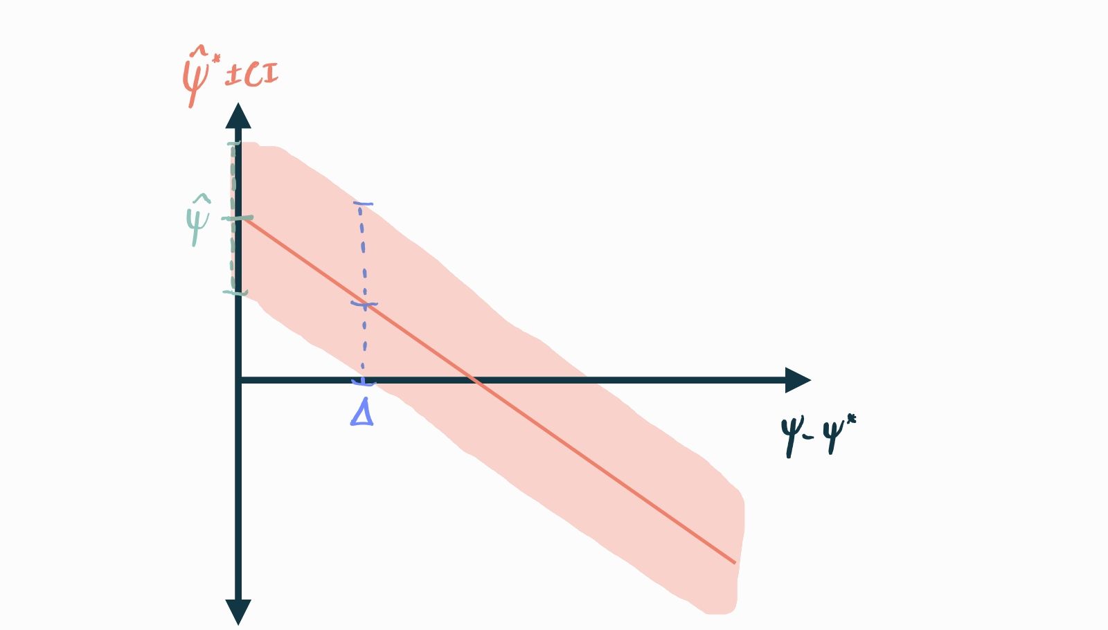
This entire exercise can just as easily be repeated in a framework where practical significance (instead of statistical) is of interest. For example, let’s say that effects of size are not of practical interest. Then perhaps it would make sense to report in our example (since the CI for would overlap ). Any information of this kind can also easily be read off of a plot like the one shown above.
In contrast to running simulations, this kind of sensitivity analysis puts the onus on the reader to posit a realistic data-generating mechanism that could attain a causal gap greater than . This could be seen as a weakness of the framework: doesn’t tell you anything specific: is our result sensitive to some kind of unobserved confounding? Is it sensitive to a positivity violation? In what subpopulation? All these questions go unanswered.
But this vagueness is also a strength: with just one plot, any stakeholder is empowered to come to the conclusion that is appropriate for their interests. The analyst is therefore not in the role of enforcing their value judgements on the reader. Moreover we don’t have to impose any assumptions at all.
Alternatives
There is a huge literature on sensitivity analyses in causal inference but you’ll find very little about purely simulation-driven methods or critical causal gaps in it. That’s because these methods are so simple and so broadly applicable that there’s really not much left to be said about them!
On the other hand, things get more “interesting” if you’re willing to work with specific problems, estimators, or make a few assumptions. Obviously if you’re willing to believe a specific parametric model you can assign a meaning to the values of different parameters and see how off your statistical parameter is from the causal parameter. But you might also try to describe part of your system nonparametrically and leave only one relevant part parametrically specified so you can test against violations of your assumptions there. There is also the question of how to quantitatively measure a violation of such an assumption (e.g. the “amount” of unmeasured confounding) without reducing it too much to a structural parameter. Basically, there is a large “gray area” between parametric simulations and a critical causal gap analysis.
The point of all this is to be able to more clearly interpret the result of the sensitivity analysis. For example, in some of these approaches, you can say things like “as long as no unobserved confounder has marginal odds ratios greater than with the outcome and treatment, then observed data support a statistically significant estimate of the causal estimand”.
Instead of taking you through a zoo of these approaches, I’ll give you a list of a few papers that you can skim to get an idea of what I mean without having to dig into all the details.
The important thing is to focus on what the restrictions are: is this method specific to a specific estimator, estimand, and/or causal model? These are often not stated explicitly! Also assess the benefits: does this method clarify how much certain assumptions can be violated vis-a-vis an agnostic causal gap analysis?
Conclusions
Partial identification and sensitivity analysis are both huge, messy fields. It can be difficult to navigate the literature and decide what to do with whatever problem you’re actually working on. Moreover, all of this requires careful consultation with domain experts who can tell you what is a reasonable assumption and what estimands are really of interest. Since it’s all a bit tricky, We’ll give you some personal guidelines- feel free to seek a second or third opinion.
First off, figure out if the causal estimand you really care about (e.g. ATE) is plausibly identified. If there is substantial doubt in the required assumptions (e.g. you know you’re missing an important confounder) then think about whether a different estimand might be identified (e.g. a complier ATE) because you have some special structure you can take advantage of in your problem (e.g. an instrument). If you can get a more defensible identification of that estimand, then go from there.
If you’re not willing to change your estimand or you can’t exploit any special structure, next see if you have enough to at least partially identify the estimand (i.e. if you can identify bounds on the estimand). There will usually be different approaches to do this that might also exploit some special structure or require particular assumptions, so review the literature and see what you can find and make use of.
If bounds aren’t good enough for you or the partial identification assumptions are themselves too complicated to defend, you should go ahead and estimate the statistical estimand you’ve got but protect yourself by doing a sensitivity analysis. We recommend a combination of a critical causal gap analysis and some simulations with semi-synthetic data since these approaches are so widely applicable and interpretable. However, if your problem has specific structure or you want a specific kind of interpretation of the sensitivity parameter, then you should go look through the literature and see if there’s something that better fits your needs.