Simulations Done Right

Alejandro Schuler

How to do Simulations

Top Tips

🎯 Thoughtful Goals = Direction!

practical utility
key insight
audience

📊 Communication = Focus!

structure + organize
minimize cognitive load

⚙️ Clean, Fast Sims = Productivity!

simple DGPs
minimize compute
modular code

🎯 Setting Goals

Setting Goals

paper = claims 🎯 + evidence
- evidence = simulations 📊, applications 🗂️, theory ♾️, etc.
A good claim likely…
- has practical utility
- builds insight
- is honest and well-scoped
Many claims are possible. Less is more! Prioritize:
- relevance to audience
- potential to change practice or thinking
sims often support claims like: “[method] works [well] when [condition] and not when [other condition]”

Exercise: TMLE

You wake up. It’s 2006. You look in the mirror and you see you are Mark van der Laan. You’ve just invented TMLE.

What are the claims you should set out for the TMLE paper? Which of them can be supported by theory and which by simulations?

Some Claims

(theory) TMLE is a general method for constructing efficient estimators of pathwise differentiable estimands
- Estimating equations already does this, so while this needs to be shown, it’s not enough to prove TMLE is useful!
TMLE is in practice “better” than…
- Plug-in estimators? AIPW is already better
- AIPW?

❓ What is meant by “better”? When should it be better and when worse?

It works in the real world? Computationally tractable, doesn’t require specific data types, etc. (usually addressable w/ theory and a single real data application)

Simulation Goals (Initial)

Across the board, AIPW and TMLE behave similarly in large samples when they have access to the same learners
TMLE is better than plugins, allowing for good coverage of Wald intervals
There are cases where TMLE is better than AIPW in small samples

Simulation Goals (Some Questions)

Across the board, AIPW and TMLE behave similarly in large samples when they have access to the same learners
- What learners?
- By what metric(s)?
Like AIPW, TMLE is better than plugins, allowing for good coverage of Wald intervals
- What learners?
- What should \(n\) be here?
- Presumably using IF-based CI
- Metric?
- But is there a way to get CIs for the plugins as a naive baseline?
There are cases where TMLE is better than AIPW in small samples
- Can we back these up with some kind of theory?
- In what DGPs?

Simulation Goals (v2)

Across the board, AIPW and TMLE behave similarly in terms of point estimate and SE estimate in large samples when they have access to the same learners
Like AIPW, TMLE improves the MSE of plugins in moderate sample sizes and allows for good coverage of Wald intervals based on IF SEs, even compared to the same SE put around the plugin
TMLE is better than AIPW in small samples when the outcome is bounded (?)

📊 Presentation

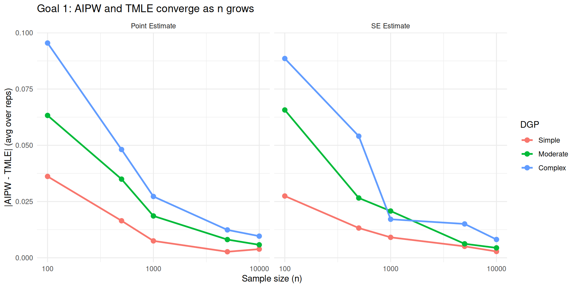
Mockup Evidence for Goal 1

Across the board, AIPW and TMLE behave similarly in terms of point estimate and SE estimate in large samples when they have access to the same learners

Mockup Evidence for Goal 2

Like AIPW, TMLE improves the MSE of plugins in moderate sample sizes and allows for good coverage of Wald intervals based on IF SEs.

Fix \(n = 300\), do \(B\) reps from the same 3 DGPs, tables like:

	plugin	AIPW	TMLE
MSE
bias
variance
coverage

One per each DGP (or 3 sub-tables). Probably just ATE, send the other estimand to the appendix.

Learners? Some fast nonparametric thing, not too relevant to goal what it is

Mockup Evidence for Goal 3

TMLE is better than AIPW in small samples when the outcome is bounded (?)

The evidence for this goal might be a subset of evidence for the above. So just suggests that one of our DGPs should have a bounded outcome, and then we can point to the relevant rows in the above table to support this claim.

Telling the Story

For each bit of evidence you present, you should tell the reader why it is there. Tell them your goal! Then give them the evidence. Then tell them how the evidence supports the goal. Be prosaic and direct.

“In the first part I tell ’em what I am going to tell ’em; in the second part — well, I tell ’em; in the third part I tell ’em what I’ve told ’em.”

Example

The point of this application is to show how fast TMLE is on a real-world dataset of size blah blah and to prove that it works with mixed datatypes, demonstrate how it can be prespecified, and produces plausible results.

ADEMP Framework

From Morris et al. (2019)

“Using simulation studies to evaluate statistical methods”

Statistics in Medicine, 38(11), 2074–2102.

Before presenting results, clearly describe:

Aims: what are the claims you are trying to support?
Data-generating mechanisms: how did you simulate the data? → DGPs
Estimands: what are the true values? → e.g. ATE() helper
Methods: what methods are you using? → ESTIMATORS
Performance measures: what metrics? → the summarize step and your tables/figures

Aims is most important, others are in service of that
This is part of the “tell them what you’re going to tell them.”
Can do separately for each claim or once

Example from a Recent Paper

arxiv.org/pdf/2503.22284

⚙️ Implementation

Advice for Machine Learning

Avoid super-learner and cross-validation
- use single-split, 1-2 good learners
Understand learners and hyperparams

ML Method Recommendations

Method	Speed	Notes
MARS (`earth`)	⚡ Super fast	Works well with a single set of hyperparams. Ensure depth is high enough, enable pruning, allow interaction.
Random forests	🏃 Fast	Works well with default hyperparams. Worse for smooth functions.
GBT (lightgbm/xgboost)	🏃 Fast	Beats almost everything. Requires tuning over # trees, depth, learning rate. Use early stopping.
Elastic net	🏃 Fast (ridge)	Loses to others with moderate nonlinearity. Good for baselines. Requires tuning regularization.
KRR (kernel ridge)	🐌 Slow	Good for smooth functions, easy to analyze theoretically. Use only for \(n < 1000\).

ML Method Recommendations

Deep learning?
- Avoid unless you specifically need a differentiable model, custom loss function, fine-tuning, etc.
- Hard to tune
- xgboost wins for tabular data.
HAL? lol. lmao even

Advice for DGPs

Being able to reason about your simulations and iterate on them is much more important than making them realistic. For example:

\(X \sim \mathsf{Unif}([-1,1]^d)\) unless otherwise required. Bounded domain helps reason about function ranges
\(A \sim \mathsf{Bern}(\text{expit}(\rho(X)))\). Keep \(\rho\) simple + sparse and, unless empirical positivity violations are your goal, shoot for \(\rho \in [-3,3]\)
\(Y \sim \mu(A, X) + \mathsf{N}(0,\sigma)\). Keep \(\mu\) simple + sparse.

Pay attention to:

positivity violations and dist of \(A|X\)
percent of outcome variance explainable by \(\mu\) (signal-to-noise ratio)
percent of variance of \(\mu\) explainable by best linear approximation

Evidence for Goal 1

Across the board, AIPW and TMLE behave similarly in terms of point estimate and SE estimate in large samples when they have access to the same learners

Settings for Goal 1

Across the board, AIPW and TMLE behave similarly in terms of point estimate and SE estimate in large samples when they have access to the same learners

What DGPs? What estimand(s)? What learners?
Do ~100 reps first, just get the vibe (do 2 reps first to see if code even runs!)
\(n\) from 100 to 10k? Start with 3–4 increments, add more later
Maybe 3 DGPs of increasing complexity/confounding. Simple \(W,A,Y\) setup w/ binary \(A\) for intelligibility. Doesn’t matter much for this goal
For convenience, choose estimands that are computationally easy and work with the same DGP, e.g. ATE and incremental pscore. Having 2 estimands helps enforce the top-level generality claim, but stick to ATE for first round of output
Learners: fast nonparametric learners for both OR and PS

Advice for Simulation Code

Separate DGPs are separate objects with draw method
Estimators are functions, separate, but can share innards
- separate out learning of common nuisances
- Generally return (est, est_se)
- Clear claims will help debug!
Simulation loop over DGPs, estimators, and reps is a simple nested loop that produces a tidy data frame of results
- Use furrr for drop-in parallelization from map in R, parallelize across reps
Keep DGPs (and helpers) in one file, estimators (and helpers) in another, and run your sims/tests in a notebook, saving results to disk as needed

DGPs: Simplest Version

library(tidyverse)
library(magrittr)

draw <- \(n) tibble(
    W1 = runif(n, -1, 1),
    W2 = runif(n, -1, 1),
    A = rbinom(n, 1, plogis(W1 + W2)),
    Y = W1 + W2 + A + rnorm(n)
)

DGPs: More Modular

rho <- \(w1, w2) w1 + w2
mu <- \(a, w1, w2) w1 + w2 + a

draw <- \(n) tibble(
    W1 = runif(n, -1, 1),
    W2 = runif(n, -1, 1),
    A = rbinom(n, 1, plogis(rho(W1, W2))),
    Y = mu(A, W1, W2) + rnorm(n)
)

DGPs: OOP Approach

simple_dgp <- structure(
    list(
        rho = \(w1, w2) w1 + w2,
        mu = \(a, w1, w2) w1 + w2 + a,
        sigma = 1
    ),
    class = "dgp"
)

complex_dgp <- structure(
    list(
        rho = \(w1, w2) w1 + w2 + w1 * abs(w2),
        mu = \(a, w1, w2) w1 + w2 + abs(w2) + 0.5 * w1 * w2,
        sigma = 1
    ),
    class = "dgp"
)

draw <- function(x, ...) UseMethod("draw")
draw.dgp <- \(dgp, n) dgp %$% tibble(
    W1 = runif(n, -1, 1),
    W2 = runif(n, -1, 1),
    A = rbinom(n, 1, plogis(rho(W1, W2))),
    Y = mu(A, W1, W2) + rnorm(n, 0, sigma)
)

draw_intervene <- function(x, ...) UseMethod("draw_intervene")
draw_intervene.dgp <- \(dgp, n, treatment) dgp %$% tibble(
    W1 = runif(n, -1, 1),
    W2 = runif(n, -1, 1),
    A = treatment(W1, W2),
    Y = mu(A, W1, W2) + rnorm(n)
)

DGPs: Usage

draw(simple_dgp, 3)

# A tibble: 3 × 4
     W1     W2     A     Y
  <dbl>  <dbl> <int> <dbl>
1 0.351  0.133     1 0.780
2 0.966  0.699     1 1.59 
3 0.519 -0.621     1 0.846

draw(complex_dgp, 3)

# A tibble: 3 × 4
      W1      W2     A     Y
   <dbl>   <dbl> <int> <dbl>
1  0.439  0.0288     1  1.26
2 -0.984 -0.997      0 -1.22
3 -0.249  0.163      1 -1.31

draw_intervene(simple_dgp, n=3, treatment = \(w1, w2) 1)

# A tibble: 3 × 4
      W1    W2     A     Y
   <dbl> <dbl> <dbl> <dbl>
1  0.335 0.866     1  1.77
2 -1.000 0.851     1  1.51
3 -0.583 0.468     1  1.21

DGP Helpers

ATE <- function(x, ...) UseMethod("ATE")
ATE.dgp <- \(dgp, n = 1e6) {
    mu0 <- dgp |> draw_intervene(n, \(w1, w2) 0) %$% mean(Y)
    mu1 <- dgp |> draw_intervene(n, \(w1, w2) 1) %$% mean(Y)
    mu1 - mu0
}

R2 <- function(x, ...) UseMethod("R2")
R2.dgp <- \(dgp, n = 1e6) {
    pop <- dgp |>
        draw(n) |>
        mutate(mu = dgp$mu(A, W1, W2))
    mu_lin <- lm(mu ~ A + W1 + W2, data = pop)
    pop <- pop |>
        mutate(mu_lin = predict(mu_lin, pop))

    list(
        R2     = pop %$% { var(mu) / var(Y) },
        R2_lin = pop %$% { var(mu_lin) / var(mu) }
    )
}

ATE(simple_dgp)

[1] 0.9990462

R2(simple_dgp)

$R2
[1] 0.5492145

$R2_lin
[1] 1

Estimators: General Structure

my_estimator <- function(
    data, # always a data frame with consistently named columns
    hyperparams_or_nuisances # whatever else you need
) {
    # computations ...

    list(
        est    = ..., # point estimate
        est_se = ...  # SE estimate
    )
}

So that it can be used like this:

dgp |> draw(100) |> my_estimator()

write code for simulation, not for a human user

Estimator: Difference in Means

diff_means <- function(data, ...) {
    data |>
        group_by(A) |>
        summarize(
            mu_hat  = mean(Y),
            var_hat = var(Y),
            n       = n()
        ) %$%
        list(
            est    = mu_hat[A == 1] - mu_hat[A == 0],
            est_se = sqrt(var_hat[A == 1] / n[A == 1] +
                          var_hat[A == 0] / n[A == 0])
        )
}

Estimators: TMLE & AIPW

library(zeallot)

tmle <- function(data, nuisances) {
    c(pi, alpha, mu) %<-% nuisances

    eps <- lm(Y - mu(A, W1, W2) ~ alpha(A, W1, W2) - 1, data) |> coef() |> unname()
    data |>
        mutate(
            mu1 = mu(1, W1, W2) + eps * alpha(1, W1, W2),
            mu0 = mu(0, W1, W2) + eps * alpha(0, W1, W2),
            phi = alpha(A, W1, W2) * (Y - mu(A, W1, W2)) + (mu1 - mu0)
        ) %$%
        list(
            est    = mean(mu1 - mu0),
            est_se = sd(phi) / sqrt(nrow(data))
        )
}

aipw <- function(data, nuisances) {
    c(pi, alpha, mu) %<-% nuisances

    data |>
        mutate(
            phi = alpha(A, W1, W2) * (Y - mu(A, W1, W2)) +
                  (mu(1, W1, W2) - mu(0, W1, W2))
        ) %$%
        list(
            est    = mean(phi),
            est_se = sd(phi) / sqrt(nrow(data))
        )
}

Learning Nuisances

library(tidymodels)

fit_learners <- function(data) {
    # Convert A to factor for classification
    data <- data |> mutate(A = factor(A))
    
    pi_obj <- mars(prod_degree = 3, num_terms = 50) |>
        set_engine("earth") |>
        set_mode("classification") |>
        fit(A ~ W1 + W2, data)

    mu_obj <- mars(prod_degree = 3, num_terms = 50) |>
        set_engine("earth") |>
        set_mode("regression") |>
        fit(Y ~ A + W1 + W2, data)

    pi    = \(w1, w2) predict(pi_obj, tibble(W1 = w1, W2 = w2), type = "prob")$.pred_1
    alpha = \(a, w1, w2) a / pi(w1, w2) -
                            (1 - a) / (1 - pi(w1, w2))
    mu    = \(a, w1, w2) predict(mu_obj, tibble(A = factor(a, levels = c(0, 1)), W1 = w1, W2 = w2))$.pred

    list(pi = pi, alpha = alpha, mu = mu)
}

Sample Splitting

# Train on a separate sample (approximation of cross-fitting,
# but much faster and less complicated)
nuisances <- simple_dgp |> draw(500) |> fit_learners()
data <- simple_dgp |> draw(500)

list(
    dm   = diff_means(data),
    tmle = tmle(data, nuisances),
    aipw = aipw(data, nuisances)
) |> map_dfr(as_tibble, .id="method")

# A tibble: 3 × 3
  method   est est_se
  <chr>  <dbl>  <dbl>
1 dm      1.47 0.110 
2 tmle    1.02 0.0955
3 aipw    1.02 0.0955

Simulation Loop

REPS <- 20
N <- 500

DGPS <- list(simple = simple_dgp, complex = complex_dgp)
ESTIMATORS <- list(dm = diff_means, tmle = tmle, aipw = aipw)

1:REPS |> map(\(rep) {
    DGPS |> imap(\(dgp, dgp_name) {
        nuisances <- dgp |> draw(N) |> fit_learners()
        data <- dgp |> draw(N)

        ESTIMATORS |> imap(\(estimator, estimator_name) {
            res <- estimator(data, nuisances)
            tibble(
                rep       = rep,
                DGP       = dgp_name,
                estimator = estimator_name,
                est       = res$est,
                se        = res$est_se
            )
        }) |> bind_rows()
    }) |> bind_rows()
}) |> bind_rows() -> results

Save the raw results object to file, possibly with a pointer to the commit hash for replicability
If you optimize runtime, you don’t have to worry so much about saving carefully since it’s so fast to regenerate!

Parallelize with `furrr`

library(furrr)
plan(multicore, workers = 10)

1:REPS |> furrr::future_map(\(rep) {
    DGPS |> imap(\(dgp, dgp_name) {
        nuisances <- dgp |> draw(N) |> fit_learners()
        data <- dgp |> draw(N)

        ESTIMATORS |> imap(\(estimator, estimator_name) {
            res <- estimator(data, nuisances)
            tibble(
                rep       = rep,
                DGP       = dgp_name,
                estimator = estimator_name,
                est       = res$est,
                se        = res$est_se
            )
        }) |> bind_rows()
    }) |> bind_rows()
}) |> bind_rows() -> results

before doing this, test with REPS = 5 and possibly fewer DGPs and estimators.
use future_map instead of map and set up a parallel plan with plan()

Analysis

true_ATEs <- DGPS |> map_dbl(ATE)

results |>
    group_by(DGP, estimator) |>
    summarize(
        bias        = mean(est - true_ATEs[DGP]),
        true_se     = sd(est),
        mean_est_se = mean(se),
        rmse        = sqrt(mean((est - true_ATEs[DGP])^2)),
        coverage    = mean(
            (est - 1.96 * se <= true_ATEs[DGP]) &
            (true_ATEs[DGP] <= est + 1.96 * se)
        )
    )

# A tibble: 6 × 7
# Groups:   DGP [2]
  DGP     estimator     bias true_se mean_est_se   rmse coverage
  <chr>   <chr>        <dbl>   <dbl>       <dbl>  <dbl>    <dbl>
1 complex aipw      -0.0137   0.0884       0.116 0.0873      1  
2 complex dm         0.663    0.105        0.115 0.671       0  
3 complex tmle      -0.00608  0.0742       0.116 0.0726      1  
4 simple  aipw      -0.0874   0.430        0.175 0.428       0.9
5 simple  dm         0.594    0.130        0.112 0.608       0  
6 simple  tmle      -0.00738  0.103        0.175 0.101       0.9

From here you can use tidyr, kable, and ggplot to make tables and figures.

Tooling Demo

Positron (files + notebook)
GitHub Copilot in Positron Assistant

What About Documentation & Testing?

Don’t bother, you’ll have to rewrite it all tomorrow
Simple comments here and there suffice
When you write a new function, unit test it in a Jupyter notebook a few times informally
GitHub? Sure. Just commit to main, don’t worry about branches, PRs, etc.

Iteration

Problem!

In your initial TMLE simulation, you find that the ML plug-in estimator outperforms TMLE and AIPW in terms of MSE. Debiasing improves bias, but at cost of variance.

Why is this bad for your claim?
What do you do?

Solution

having a clear goal made it easy to know if result was “good” or “bad”
understand theory: why is debiasing necessary?
modify claim:

Like AIPW, TMLE improves the MSE of plugins in moderate sample sizes when overlap is reasonable and initial estimates are biased and allows for good coverage of Wald intervals based on IF SEs.

Simulations Done Right

How to do Simulations

Top Tips

🎯 Thoughtful Goals = Direction!

📊 Communication = Focus!

⚙️ Clean, Fast Sims = Productivity!

🎯 Setting Goals

Setting Goals

Exercise: TMLE

Some Claims

Simulation Goals (Initial)

Simulation Goals (Some Questions)

Simulation Goals (v2)

📊 Presentation

Mockup Evidence for Goal 1

Mockup Evidence for Goal 2

Mockup Evidence for Goal 3

Telling the Story

ADEMP Framework

Example from a Recent Paper

⚙️ Implementation

Advice for Machine Learning

ML Method Recommendations

ML Method Recommendations

Advice for DGPs

Evidence for Goal 1

Settings for Goal 1

Advice for Simulation Code

DGPs: Simplest Version

DGPs: More Modular

DGPs: OOP Approach

DGPs: Usage

DGP Helpers

Estimators: General Structure

Estimator: Difference in Means

Estimators: TMLE & AIPW

Learning Nuisances

Sample Splitting

Simulation Loop

Parallelize with furrr

Analysis

Tooling Demo

What About Documentation & Testing?

Iteration

Problem!

Solution

Conclusions

How to do Simulations

Top Tips

🎯 Thoughtful Goals = Direction!

📊 Communication = Focus!

⚙️ Clean, Fast Sims = Productivity!

Parallelize with `furrr`