Functional Programming
Learning Goals:
- write and test your own functions
- iterate functions over lists of arguments
Writing functions
Motivation
- It’s handy to be able to reuse your code and automate repetitive tasks
- Writing your own functions allows you to do that
- When you write your code as functions, you can
- name the function something evocative and readable
- update the code in a single place instead of many
- reduce the chance of making mistakes while copy-pasting
- make your code shorter overall
What does this code do? (note that df$col is a shortcut for df |> pull(col))
df$a = (df$a - min(df$a, na.rm = TRUE)) /
  (max(df$a, na.rm = TRUE) - min(df$a, na.rm = TRUE))
df$b = (df$b - min(df$b, na.rm = TRUE)) /
  (max(df$b, na.rm = TRUE) - min(df$a, na.rm = TRUE))
df$c = (df$c - min(df$c, na.rm = TRUE)) /
  (max(df$c, na.rm = TRUE) - min(df$c, na.rm = TRUE))
df$d = (df$d - min(df$d, na.rm = TRUE)) /
(max(df$d, na.rm = TRUE) - min(df$d, na.rm = TRUE))- It looks like we’re standardizing all the variables by their range so that they fall between 0 and 1
- But did you spot the mistake? The code runs with no errors…
- Much improved!
- The last two lines clearly say: replace all the columns with their rescaled versions
- This is because the function name
rescale()is informative and communicates what it does - If a user (or you a few weeks later) is curious about the specifics, they can check the function body
- This is because the function name
- Even better.
- … now we notice that
min()is being computed twice in the function body, which is inefficient - We are also not accounting for NAs
- Since we have a function, we can make the change in a single place and improve the efficiency of multiple parts of our code
- Bonus question: why use
range()instead of getting and saving the results ofmin()andmax()separately?
We can also test our function in cases where we know what the output should be to make sure it works as intended before we let it loose on the real data
[1] 0 0 0 0 0 1 [1] 0.0 0.1 0.2 0.3 0.4 0.5 0.6 0.7 0.8 0.9 1.0 [1] 0.0 0.1 0.2 0.3 0.4 0.5 0.6 0.7 0.8 0.9 1.0[1] TRUE- These tests are a critical part of writing good code! It is helpful to save your tests in a separate file and organize them as you go
Function declaration syntax
To write a function, just wrap your code in some special syntax that tells it what variables will be passed in and what will be returned
- Just like assigning a variable, except what you put into
FUNCTION_NAMEnow isn’t a data frame, vector, etc, it’s a function object that gets created by thefunction(..) {...}syntax - At any point in the body you can
return()the value, or R will automatically return the result of the last line of code in the body that gets run - once declared, it can be called:
- The syntax is
FUNCTION_NAME <- function(ARGUMENTS...) { CODE } - what you call the arguments that go in the
function(...)part is how the function will refer to these inputs internally and specify how it should be called using named arguments

aes = function(x,y) {...} # defining
aes(x=EIF3L, y=VAPA) # calling
Optional arguments
To add an optional argument, add an = after you declare it as a variable and write in the default value that you would like that variable to take
rescale = function(x, na.rm=TRUE) {
  x_rng = range(x, na.rm=na.rm)
  (x - x_rng[1])/(x_rng[2] - x_rng[1])
}

vec = c(0,1,NA)

rescale(vec)
[1] 0 1 NA[1] 0 1 NA[1] NA NA NA- All optional arguments must go after mandatory arguments in the function declaration
Exercise: Reverse
- write a function that takes a single vector or list as input and returns it in reverse order
Exercise: Hardcoding na.rm
type:prompt - It’s annoying that the sum() function returns NA if any values of the input vector are NA. You can fix this by passing in the optional argument na.rm=T every time you call sum(), but it’s inconvenient to type that every single time. - Write a new function (called sum_obs(), short for “sum observed”) that takes a vector and returns the sum of all the non-NA values. Your function should call the usual sum() internally.
Exercise: NAs in two vectors
type: prompt - Write a function called both_na() that takes two vectors of the same length and returns the total number of positions that have an NA in both vectors - Make a few vectors and test out your code
Returning multiple values
- A function can only return a single object
- Often, however, it makes sense to group the calculation of two or more things you want to return within a single function
- You can put all of that into a list and then return a single list
- Why might this code be preferable to running
min()and thenmax()?
Functions are objects
function(x, na.rm=TRUE) {
  x_rng = range(x, na.rm=na.rm)
  (x - x_rng[1])/(x_rng[2] - x_rng[1])
}
<bytecode: 0x126031510>- Because of this, they themselves can be passed as arguments to other functions
- This is what functional programming means. The functions themselves are can be treated as regular objects like variables
- The name of the function is just what you call the “box” that the function (the code) lives in, just like variables names are names for “boxes” that contain data
Iteration
Map
- Map is a function that takes a list (or vector) as its first argument and a function as its second argument
- Recall that functions are objects just like anything else so you can pass them around to other functions
- Map then runs that function on each element of the first argument, slaps the results together into a list, and returns that
- as another example, let’s say you want to read in multiple files:
Exercise: map practice
data_frames is a list of three data frames. Use map to output:
- the number of rows of each data frame
- the number of columns of each data frame
Why not for loops?
- R also provides something called a
forloop, which is common to many other languages as well. It looks like this:
- The
forloop is very flexible and you can do a lot with it forloops are unavoidable when the result of one iteration depends on the result of the last iteration
- Compare to the
map()-style solution:
- Compared to the
forloop, themap()syntax is much more concise and eliminates much of the “admin” code in the loop (setting up indices, initializing the list that will be filled in, indexing into the data structures) - The
map()syntax also encourages you to write a function for whatever is happening inside the loop. This means you have something that’s reusable and easily testable, and your code will look cleaner - Loops in R can be catastrophically slow due to the complexities of copy-on-modify semantics.
Anonymous function syntax
- up until now we had to define our functions outside of map and then pass them in as an argument:
- Instead, we can define a function inside of another function call.
- These functions are “anonymous” because they are never assigned a name and will not be used again
- the syntax is
\(ARGUMENTS) BODY - just an abbreviation for
function(ARGUMENTS) {BODY}
Exercise: read files
Earlier we saw this example of reading in multiple files:
- modify the code so that only the first 10 lines of each file are read in.
Returning other data types
map()typically returns a list (why?)- But there are variants that return different data types
Exercise: simulation
My friend is interested in whther people prefer vanilla or chocolate ice cream in San Francisco so he survyed 20 random people, 14 of which preferred vanilla. Based on the overwhelming majority in the survey, he concludes that most people in SF like vanilla.
Could he be wrong? Is it possible he got a lucky (or unlucky) sample and would have gotten a different answer if he repeated his survey? Let’s presume that, in reality, only 49% of people prefer vanilla (in other words, most people actually like chocolate and my friend is wrong). If we could observe that data it would look like this:
- Write a function that has no arguments which takes 20 random rows from this dataframe and returns whether the majority in that sample prefer vanilla (
TRUEorFALSE). This simulates my friend’s survey. - Use
mapto run this function 500 times (hint: pass 1:500 as the first argument tomap) and record all the results as a logical vector - Take the average of the resulting logical vector to see how likely it is to get vanilla as the preferred answer in a 20-person survey even if the population preference is actually chocolate!
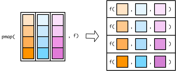
Mapping over multiple inputs
- So far we’ve mapped along a single input. But often you have multiple related inputs that you need iterate along in parallel. That’s the job of
pmap(). For example, imagine you want to draw a random numbers betweenaandbas both of those vary:
Mapping over names
imap()lets you operate on the names of the input list.
$class_A
# A tibble: 5 × 2
  grade class
  <dbl> <chr>
1    90 class_A
2    87 class_A
3    92 class_A
4    78 class_A
5    69 class_A

$class_B
# A tibble: 7 × 2
  grade class
  <dbl> <chr>
1    88 class_B
2    85 class_B
3    76 class_B
4    78 class_B
5    77 class_B
6    97 class_B
7    91 class_B
Creating a grid of values
expand_grid()gives you every combination of the items in the list you pass it
Exercise: dimensions
Fill in the missing parts of the code below to programmatically create the following table:
Error: The pipe operator requires a function call as RHS (<text>:8:3)Exercise: reading files in multiple directories
My collaborator has an online folder of experimental results named results that can be found at "https://raw.githubusercontent.com/alejandroschuler/r4ds-courses/summer-2023/data/results". In that folder, there are 20 sub-folders that represent the results of each repetition of her experiment. These sub-folders are each named rep_n, so, e.g. results/rep_14 would be one sub-folder. Within each sub-folder, there are 3 csv files called a.csv, b.csv c.csv that contain different kinds of measurements. Thus, a full path to one of these files might be results/rep_14/c.csv.
write code to read these all into one long list of data frames.
str_c()orglue()will be helpful to create the required file namesUnfortunately, that wasn’t helpful because now you don’t know what data frames are what results. Consider just the “
a” files. Write code that reads in only the “a” files and concatenates them into one data frame. Include a column in this data frame that indicates which experimental repetition each row of the data frame came from (useimap()).Turn your code from above into a function that takes as input the file name (
'a', for example) and returns the single concatenated file. Iterate that function over the different file names to output three master data frames corresponding to the file types'a','b', and'c'.