Advanced Tabular Data

Alejandro Schuler

Learning Goals:

• group and summarize data by one or more columns
• transform between long and wide data formats
• combine multiple data frames using joins on one or more columns

Summaries

GTEx data

This is a subset of the Genotype Tissue Expression (GTEx) dataset

• The full dataset. Includes gene expression data, measured via RNA-sequencing, from 54 post-mortem tissues in ~800 individuals. Whole genome sequencing is also available for these individuals as part of the GTEx v8 release, available through dbGaP.
• The subsetted dataset. We are looking at expression data for just 78 individuals here, in four tissues including blood, heart, lung and liver.
• Data processing The expression values have been normalized and corrected for technical covariates and are now in the form of “Z-scores”, which indicate the distance of a given expression value from the mean across all measurements of that gene in that tissue.
• Goal. We will use the data here to illustrate different functions for data transformation, often focused on extracting individuals with extremely high or low expression values for a given gene as compared to the distribution across all samples.

# Read subsetted data from online file - make sure there are no spaces
gtex = read_tsv('https://tinyurl.com/342rhdc2')

# Check number of rows
nrow(gtex)

[1] 389922

Summarize

summarize(gtex, blood_avg=mean(Blood, na.rm=T))

# A tibble: 1 × 1
  blood_avg
      <dbl>
1 -0.000435

• summarize() boils down the data frame according to the conditions it gets. In this case, it creates a data frame with a single column called blood_avg that contains the mean of the Blood column
• As with mutate(), the name on the left of the = is something you make up that you would like the new column to be named.
• mutate() transforms columns into new columns of the same length, but summarize() collapses down the data frame into a single row

• note that you can also pass in multiple conditions that operate on multiple columns at the same time

gtex |> 
summarize( # newlines not necessary, again just increase clarity
  lung_avg = mean(Lung, na.rm=T),
  blood_max = max(Blood, na.rm=T),
  blood_lung_dif_min = min(Blood - Lung, na.rm=T)
)

# A tibble: 1 × 3
  lung_avg blood_max blood_lung_dif_min
     <dbl>     <dbl>              <dbl>
1  0.00233      18.9              -12.8

Exercise: summaries

Find the average, maximum, and minimum expressions of the REN gene in blood. Hint: filter and summarize.

Grouping

Grouped summaries

• Summaries are more useful when you apply them to subgroups of the data

gtex |> 
  group_by(Gene) |>
  summarize(max_blood = max(Blood))

# A tibble: 4,999 × 2
   Gene               max_blood
   <chr>                  <dbl>
 1 A2ML1                   2.08
 2 A3GALT2                 2.77
 3 A4GALT                  2.78
 4 AAMDC                  NA   
 5 AANAT                   1.71
 6 AAR2                    2.52
 7 AARSD1                  1.89
 8 AB019441.29             2.31
 9 ABC7-42389800N19.1      1.98
10 ABCA5                   2.3 
# ℹ 4,989 more rows

• group_by() is a helper function that “groups” the data according to the unique values in the column(s) it gets passed.

• Its output is a grouped data frame that looks the same as the original except for some additional metadata that subsequent functions can use
• summarize() works the same as before, except now it returns as many rows as there are groups in the data
• The result also always contains colunmns corresponding to the unique values of the grouping variable

Group on many columns

gtex |> 
  filter(!is.na(Blood) & !is.na(Lung)) |>
  group_by(
    pos_blood = Blood>0, 
    pos_lung = Lung>0
  ) |>
  summarize(mean_liver = mean(Liver, na.rm=T))

# A tibble: 4 × 3
# Groups:   pos_blood [2]
  pos_blood pos_lung mean_liver
  <lgl>     <lgl>         <dbl>
1 FALSE     FALSE       -0.106 
2 FALSE     TRUE         0.0145
3 TRUE      FALSE       -0.0141
4 TRUE      TRUE         0.109 

• The result has the summary value for each unique combination of the grouping variables

Computing the number of rows in each group

• The n() function counts the number of rows in each group:

gtex |> 
  filter(!is.na(Blood)) |>
  group_by(Gene) |>
  summarize(how_many = n())

# A tibble: 4,999 × 2
   Gene               how_many
   <chr>                 <int>
 1 A2ML1                    78
 2 A3GALT2                  78
 3 A4GALT                   78
 4 AAMDC                    77
 5 AANAT                    78
 6 AAR2                     78
 7 AARSD1                   78
 8 AB019441.29              78
 9 ABC7-42389800N19.1       78
10 ABCA5                    78
# ℹ 4,989 more rows

• You can also use count(), which is just a shorthand for the same thing

gtex |> 
  filter(!is.na(Blood)) |>
  group_by(Gene) |>
  count()

Exercise: expression range per gene

Ignoring NAs, what are the highest and lowest liver expression values seen for each gene in the gtex dataset?

1. What steps should you take to solve this problem? When you have a question that asks something about “for each …” that usually indicates that you need to group_by() the data by whatever thing that is. When you are asking about a summary measure (like a mean, max etc.), that usually indicates the use of summarize(). In this problem, what column(s) are you grouping by? What summaries of what columns are you computing?

2. Now that you have a structure, write the code to implement it and solve the problem.

Exercise: summarize and plot

Before continuing, run this code to reformat your data and store it as a new data frame gtex_tidy (we’ll see how to do this later today):

gtex_tidy = gtex |>
  pivot_longer(
    Blood:Liver, 
    names_to="tissue",
    values_to="expression"
  )

Have a look at the dataframe you created. Use it to recreate this plot:

The max_expression variable in the x-axis of the plot indicates the maximum expression across all samples (in whatever grouping we are looking at).

It’s helpful to think backwards from the output you want. First outline the ggplot code that would generate the given plot. What does the dataset need to look like that is going into ggplot in order to get the plot shown here? How can we get from gtex_tidy to that data?

Filtering grouped data

• filter() is aware of grouping. When used on a grouped dataset, it applies the filtering condition separately in each group

gtex |>
  select(Ind, Gene, Lung) |>
  group_by(Ind) |>
  filter(Lung == max(Lung, na.rm=T))

# A tibble: 79 × 3
# Groups:   Ind [78]
   Ind        Gene          Lung
   <chr>      <chr>        <dbl>
 1 GTEX-11TUW AC007743.1    4.32
 2 GTEX-147F4 ACRV1         5.4 
 3 GTEX-YFC4  ALOXE3        7.5 
 4 GTEX-ZPU1  ANKDD1B       4.12
 5 GTEX-X4EP  AP001610.5    6.59
 6 GTEX-1GN2E ATF4P3        6.95
 7 GTEX-1LGRB CASP12        3.66
 8 GTEX-1E2YA COLGALT1      6.96
 9 GTEX-17HGU CTAG2         7.4 
10 GTEX-14E1K CTD-2525I3.5  5.9 
# ℹ 69 more rows

• This is an extremely convenient idiom for finding the rows that minimize or maximize a condition

Mutating grouped data

gtex |>
  group_by(Gene) |>
  mutate(rank = rank(-Blood)) |>
  select(Gene, Ind, rank, Blood) |>
  filter(rank <= 3) |>
  arrange(Gene, rank)

# A tibble: 14,867 × 4
# Groups:   Gene [4,999]
   Gene    Ind         rank Blood
   <chr>   <chr>      <dbl> <dbl>
 1 A2ML1   GTEX-1A8FM     1  2.08
 2 A2ML1   GTEX-WY7C      2  1.73
 3 A2ML1   GTEX-ZTPG      3  1.11
 4 A3GALT2 GTEX-1AX9I     1  2.77
 5 A3GALT2 GTEX-14XAO     2  1.54
 6 A3GALT2 GTEX-1B933     3  1.41
 7 A4GALT  GTEX-12696     1  2.78
 8 A4GALT  GTEX-18A6Q     2  2.66
 9 A4GALT  GTEX-11DXZ     3  2.02
10 AAMDC   GTEX-14XAO     1  2.32
# ℹ 14,857 more rows

• when mutate is used on a grouped dataset, it applies the mutation separately in each group

gtex |>
  mutate(rank = rank(-Blood)) |>
  select(Gene, Ind, rank, Blood) |>
  filter(rank <= 3) |>
  arrange(Gene, rank)

# A tibble: 3 × 4
  Gene    Ind         rank Blood
  <chr>   <chr>      <dbl> <dbl>
1 DNASE2B GTEX-12696     3  14.4
2 KLK3    GTEX-147F4     2  15.7
3 REN     GTEX-U8XE      1  18.9

• without the group_by, the ranking is done overall across all genes.

Exercise: Max expression blood and lung

Create a dataset that shows which gene has the lowest expression in each person’s heart tissue

Tidy data: rearranging a data frame

Messy data

• Sometimes data are organized in a way that makes it difficult to compute in a vector-oriented way. For example, look at this dataset:

gtex_time_tissue_data = read_csv("https://tinyurl.com/3wd4dcsf")

head(gtex_time_tissue_data, 3)

# A tibble: 3 × 8
  tissue         `2011` `2012` `2013` `2014` `2015` `2016` `2017`
  <chr>           <dbl>  <dbl>  <dbl>  <dbl>  <dbl>  <dbl>  <dbl>
1 Adipose Tissue     56    107    243    206     84    134      2
2 Adrenal Gland      28     41     84     65     20     31      0
3 Bladder             2     18      0      1      0      0      0

• the values in the table represent how many samples of that tissue were collected during that year.
• How could I use ggplot to make this plot? It’s hard!

Messy data

head(gtex_time_tissue_data, 3)

# A tibble: 3 × 8
  tissue         `2011` `2012` `2013` `2014` `2015` `2016` `2017`
  <chr>           <dbl>  <dbl>  <dbl>  <dbl>  <dbl>  <dbl>  <dbl>
1 Adipose Tissue     56    107    243    206     84    134      2
2 Adrenal Gland      28     41     84     65     20     31      0
3 Bladder             2     18      0      1      0      0      0

• One of the problems with the way these data are formatted is that the year collected, which is a property of the samples, is stuck into the names of the columns.
• Because of this, it’s also not obvious what the numbers in the table mean (although we know they are counts)

Tidy data

• Here’s a better way to organize the data:

# A tibble: 6 × 3
  tissue         year  count
  <chr>          <chr> <dbl>
1 Adipose Tissue 2011     56
2 Adipose Tissue 2012    107
3 Adipose Tissue 2013    243
4 Adipose Tissue 2014    206
5 Adipose Tissue 2015     84
6 Adipose Tissue 2016    134

This data is tidy. Tidy data follows three precepts:

1. each “variable” has its own dedicated column
2. each “observation” has its own row
3. each type of observational unit has its own data frame

In our example, each of the observations are different groups of samples, each of which has an associated tissue, year, and count. These are the variables that are associated with the groups of samples.

Tidy data

Tidy data is easy to work with.

tidy |> 
  filter(tissue %in% c("Blood", "Heart", "Liver", "Lung")) |>
  ggplot() +
  geom_bar(aes(x = year, y = count, fill = tissue), stat = 'identity')

Tidying data with pivot_longer()

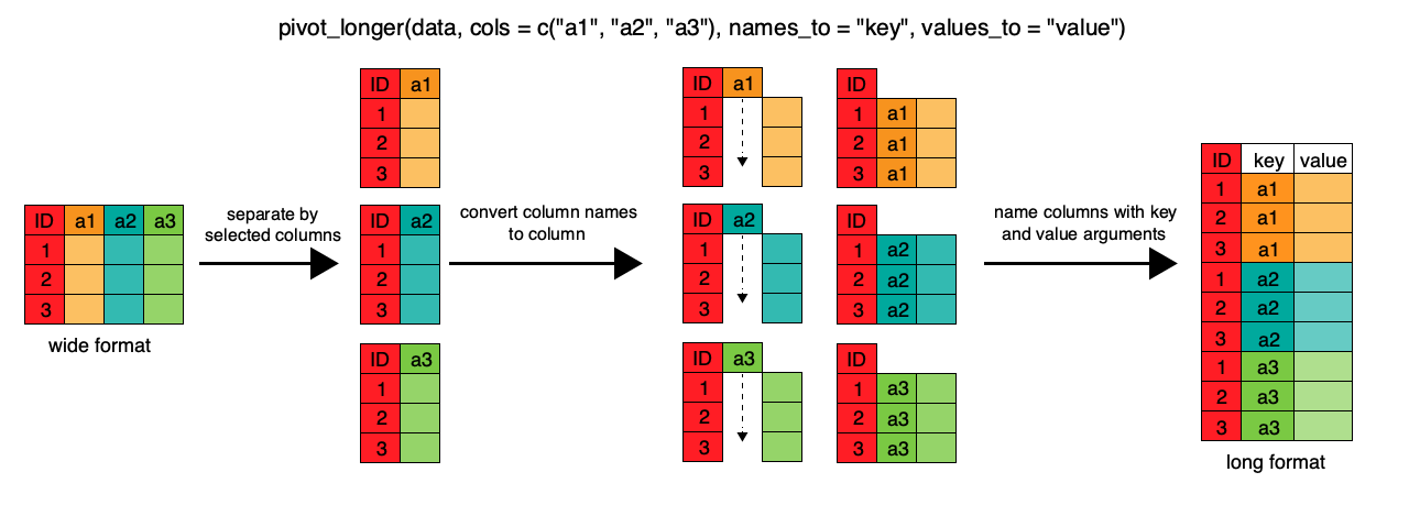
• tidyr::pivot_longer() is the function you will most often want to use to tidy your data
• the three important arguments are: a) a selection of columns, b) the name of the new key column, and c) the name of the new value column

Tidying data with pivot_longer()

• tidyr::pivot_longer() is the function you will most often want to use to tidy your data

gtex_time_tissue_data |>
  pivot_longer(-tissue, names_to = "year", values_to = "count") |>
  head(2)

# A tibble: 2 × 3
  tissue         year  count
  <chr>          <chr> <dbl>
1 Adipose Tissue 2011     56
2 Adipose Tissue 2012    107

• the three important arguments are: a) a selection of columns, b) the name of the new key column, and c) the name of the new value column

“Messy” data is relative and not always bad

# A tibble: 4 × 3
  mouse weight_before weight_after
  <dbl>         <dbl>        <dbl>
1     1         10.5          9.92
2     2          5.92         7.28
3     3          8.03        14.1 
4     4         10.5          9.99

wide_mice |>
  mutate(weight_gain = weight_after - weight_before) |>
  select(mouse, weight_gain)

# A tibble: 4 × 2
  mouse weight_gain
  <dbl>       <dbl>
1     1      -0.614
2     2       1.36 
3     3       6.03 
4     4      -0.485

# A tibble: 8 × 3
  mouse time   weight
  <dbl> <chr>   <dbl>
1     1 before  10.5 
2     1 after    9.92
3     2 before   5.92
4     2 after    7.28
5     3 before   8.03
6     3 after   14.1 
7     4 before  10.5 
8     4 after    9.99

long_mice |>
  group_by(mouse) |>
  mutate(weight_gain = weight - lag(weight)) |>
  filter(!is.na(weight_gain)) |>
  select(mouse, weight_gain)

# A tibble: 4 × 2
# Groups:   mouse [4]
  mouse weight_gain
  <dbl>       <dbl>
1     1      -0.614
2     2       1.36 
3     3       6.03 
4     4      -0.485

Pivoting wider

• As we saw with the mouse example, sometimes our data is actually easier to work with in the “wide” format.
• wide data is also often nice to make tables for presentations, or is (unfortunately) sometimes required as input for other software packages
• To go from long to wide, we use pivot_wider():

long_mice

# A tibble: 8 × 3
  mouse time   weight
  <dbl> <chr>   <dbl>
1     1 before  10.5 
2     1 after    9.92
3     2 before   5.92
4     2 after    7.28
5     3 before   8.03
6     3 after   14.1 
7     4 before  10.5 
8     4 after    9.99

long_mice |> 
  pivot_wider(
    names_from = time, 
    values_from = weight
  )

# A tibble: 4 × 3
  mouse before after
  <dbl>  <dbl> <dbl>
1     1  10.5   9.92
2     2   5.92  7.28
3     3   8.03 14.1 
4     4  10.5   9.99

Exercise: pivot

I have a dataset that records the pollution levels (in ppm) in three cities across five months:

pollution = read_csv(
  "https://tinyurl.com/yu983bhc"
)
pollution

# A tibble: 15 × 3
   city  month smoke_ppm
   <chr> <chr>     <dbl>
 1 SF    Jan       14.4 
 2 SF    Feb       39.4 
 3 SF    Mar       20.4 
 4 SF    Apr       44.2 
 5 SF    May       47.0 
 6 LA    Jan        2.28
 7 LA    Feb       26.4 
 8 LA    Mar       44.6 
 9 LA    Apr       27.6 
10 LA    May       22.8 
11 NY    Jan       47.8 
12 NY    Feb       22.7 
13 NY    Mar       33.9 
14 NY    Apr       28.6 
15 NY    May        5.15

Use a pivot and mutate to compute the difference in pollution levels between SF and LA across all 5 months. The output should look like this:

# A tibble: 5 × 4
  month    SF    LA SF_LA_diff
  <chr> <dbl> <dbl>      <dbl>
1 Jan    14.4  2.28       12.1
2 Feb    39.4 26.4        13.0
3 Mar    20.4 44.6       -24.2
4 Apr    44.2 27.6        16.6
5 May    47.0 22.8        24.2

Exercise: cleaning GTEX

Use the GTEX data to reproduce the following plot:

The individuals and genes of interest are c('GTEX-11GSP', 'GTEX-11DXZ') and c('A2ML1', 'A3GALT2', 'A4GALT'), respectively.

Think backwards: what do the data need to look like to make this plot? How do we pare down and reformat gtex so that it looks like what we need?

Exercise: tabulating missigness

Use the GTEX data to make the following table:

[1] "Number of missing tissues:"

# A tibble: 2 × 4
# Groups:   Ind [2]
  Ind        A2ML1 A3GALT2 A4GALT
  <chr>      <int>   <int>  <int>
1 GTEX-11DXZ     1       0      0
2 GTEX-11GSP     0       0      0

The numbers in the table are the number of tissues in each individual for which the gene in question was missing.

Combining multiple tables with joins

Relational data

• When we get an expression dataset, the data is usually divided into an expression matrix with the expression values of each sample, and table(s) with metadata about the samples themselves.

gtex_samples = read_csv("https://tinyurl.com/2hy9awda")
gtex_subjects = read_csv("https://tinyurl.com/3tfbew8f")
gtex_batches = read_csv("https://tinyurl.com/3phsbxsj")

• The sample data has information about the tissue and the subject who contributed the sample, the batch it was processed in, the center the sample was processed at, and the RNA integrity number (RIN score) for the sample.

gtex_samples |> head(1)

# A tibble: 1 × 6
  subject_id sample_id     batch_id center_id tissue rin_score
  <chr>      <chr>         <chr>    <chr>     <chr>      <dbl>
1 GTEX-11DXZ 0003-SM-58Q7X BP-39216 B1        Blood         NA

• The subject data table contains some subject demographic information.

gtex_subjects |> head(1)

# A tibble: 1 × 4
  subject_id sex   age   death     
  <chr>      <chr> <chr> <chr>     
1 GTEX-11DXZ male  50-59 ventilator

• The batch data contains the batch type and the dates the batches were run

gtex_batches |> head(1)

# A tibble: 1 × 3
  batch_id batch_type                                         batch_date
  <chr>    <chr>                                              <chr>     
1 BP-38516 DNA isolation_Whole Blood_QIAGEN Puregene (Manual) 05/02/2013

• These data are not independent of each other. Subjects described in the subject data are referenced in the sample data, and the batches referenced in the sample data are in the batch data. The sample ids from the sample data are used for accessing expression data.

• subject connects to sample via a single variable, subject_id.
• sample connects to batch through the batch_id variable.

An example join

• Imagine we want to add subject information to the sample data
• We can accomplish that with a join:

gtex_samples |> 
  inner_join(gtex_subjects, by = join_by(subject_id))

# A tibble: 312 × 9
   subject_id sample_id    batch_id center_id tissue rin_score sex   age   death
   <chr>      <chr>        <chr>    <chr>     <chr>      <dbl> <chr> <chr> <chr>
 1 GTEX-11DXZ 0003-SM-58Q… BP-39216 B1        Blood       NA   male  50-59 vent…
 2 GTEX-11DXZ 0126-SM-5EG… BP-44460 B1        Liver        7.9 male  50-59 vent…
 3 GTEX-11DXZ 0326-SM-5EG… BP-44460 B1        Heart        8.3 male  50-59 vent…
 4 GTEX-11DXZ 0726-SM-5N9… BP-43956 B1        Lung         7.8 male  50-59 vent…
 5 GTEX-11GSP 0004-SM-58Q… BP-39412 B1        Blood       NA   fema… 60-69 sudd…
 6 GTEX-11GSP 0626-SM-598… BP-44902 B1        Liver        6.2 fema… 60-69 sudd…
 7 GTEX-11GSP 0726-SM-598… BP-44902 B1        Lung         6.9 fema… 60-69 sudd…
 8 GTEX-11GSP 1226-SM-598… BP-44902 B1        Heart        7.9 fema… 60-69 sudd…
 9 GTEX-11NUK 0004-SM-58Q… BP-39723 B1        Blood       NA   male  50-59 sudd…
10 GTEX-11NUK 0826-SM-5HL… BP-43730 B1        Lung         7.4 male  50-59 sudd…
# ℹ 302 more rows

Joins

x = tibble(
  key = c(1, 2, 3),
  val_x = c("x1", "x2", "x3")
)

y = tibble(
  key = c(1, 2, 4),
  val_y = c("y1", "y2", "y3")
)

inner_join(x, y, by = join_by(key))

# A tibble: 2 × 3
    key val_x val_y
  <dbl> <chr> <chr>
1     1 x1    y1   
2     2 x2    y2   

• An inner join matches pairs of observations when their “keys” are equal
• the column that is joined on is specified as a “key” with the argument by=join_by(column_name)

Joins: a simple example

band_members

# A tibble: 3 × 2
  name  band   
  <chr> <chr>  
1 Mick  Stones 
2 John  Beatles
3 Paul  Beatles

band_instruments

# A tibble: 3 × 2
  name  plays 
  <chr> <chr> 
1 John  guitar
2 Paul  bass  
3 Keith guitar

inner_join(
  band_instruments, 
  band_members
)

# A tibble: 2 × 3
  name  plays  band   
  <chr> <chr>  <chr>  
1 John  guitar Beatles
2 Paul  bass   Beatles

full_join(
  band_instruments, 
  band_members
)

# A tibble: 4 × 3
  name  plays  band   
  <chr> <chr>  <chr>  
1 John  guitar Beatles
2 Paul  bass   Beatles
3 Keith guitar <NA>   
4 Mick  <NA>   Stones 

Duplicate keys

x = tibble(
  key = c(1, 2, 2, 3),
  val_x = c("x1", "x2", "x3", "x4")
)

y = tibble(
  key = c(1, 2, 2, 4),
  val_y = c("y1", "y2", "y3", "y4")
)

inner_join(x, y, join_by(key))

# A tibble: 5 × 3
    key val_x val_y
  <dbl> <chr> <chr>
1     1 x1    y1   
2     2 x2    y2   
3     2 x2    y3   
4     2 x3    y2   
5     2 x3    y3   

When keys are duplicated, multiple rows can match multiple rows, so each possible combination is produced

Specifying the keys

gtex_samples |> 
  inner_join(gtex_subjects, join_by(center_id))

Error in `inner_join()`:
! Join columns in `y` must be present in the data.
✖ Problem with `center_id`.

• Why does this fail?

• When keys have different names in different dataframes, the syntax to join is:

head(gtex, 2)

# A tibble: 2 × 6
  Gene  Ind        Blood Heart  Lung Liver
  <chr> <chr>      <dbl> <dbl> <dbl> <dbl>
1 A2ML1 GTEX-11DXZ -0.14 -1.08 NA    -0.66
2 A2ML1 GTEX-11GSP -0.5   0.53  0.76 -0.1 

head(gtex_subjects, 2)

# A tibble: 2 × 4
  subject_id sex    age   death                    
  <chr>      <chr>  <chr> <chr>                    
1 GTEX-11DXZ male   50-59 ventilator               
2 GTEX-11GSP female 60-69 sudden but natural causes

gtex |> 
  inner_join(gtex_subjects, join_by(Ind == subject_id)) |> 
  head(5)

# A tibble: 5 × 9
  Gene  Ind        Blood Heart  Lung Liver sex    age   death                   
  <chr> <chr>      <dbl> <dbl> <dbl> <dbl> <chr>  <chr> <chr>                   
1 A2ML1 GTEX-11DXZ -0.14 -1.08 NA    -0.66 male   50-59 ventilator              
2 A2ML1 GTEX-11GSP -0.5   0.53  0.76 -0.1  female 60-69 sudden but natural caus…
3 A2ML1 GTEX-11NUK -0.08 -0.4  -0.26 -0.13 male   50-59 sudden but natural caus…
4 A2ML1 GTEX-11NV4 -0.37  0.11 -0.42 -0.61 male   60-69 sudden but natural caus…
5 A2ML1 GTEX-11TT1  0.3  -1.11  0.59 -0.12 male   20-29 ventilator              

Note that the first key (Ind) corresponds to the first data frame (gtex) and the second key (subject_id) corresponds to the second data frame (gtex_subjects).

Exercise: join

How does the average A2ML1 expression in lung tissue compare between females vs. males? To answer this question let’s break it down:

1. Since we only care about A2ML1, we can start by filtering gtex to only include those rows.
2. To add sex information for each subject, we have to join our result to the gtex_subjects data frame.
3. Finally, we can group that result by sex and summarize the average expression in lung tissue.

Write the code to execute these steps.

Exercise: finding expression of specific samples

Use joins to find the samples collected in 2015 with blood expression greater than 3 of “KRT19” in males. Start with the batch_data_year; this data has an extra extracted column with the year.

batch_data_year = 
  gtex_batches |> 
  mutate(
    batch_date = lubridate::mdy(batch_date), 
    year = lubridate::year(batch_date)
  ) 

head(batch_data_year, 2)

# A tibble: 2 × 4
  batch_id batch_type                                         batch_date  year
  <chr>    <chr>                                              <date>     <dbl>
1 BP-38516 DNA isolation_Whole Blood_QIAGEN Puregene (Manual) 2013-05-02  2013
2 BP-42319 RNA isolation_PAXgene Tissue miRNA                 2013-08-14  2013

Start by figuring out what other data frame(s) you have to join to. Consider also what other operations you must do to pick out the data of interest and in what order (if it matters).

Exercise: join vs. concatenation

Another common way to combine two data frames is bind_rows (or bind_cols). Read the documentation for those functions and compare to what you know about joins. What is fundamentally different about binding (concatenating) vs. joining?

When would you do one vs. the other?

Joining on multiple columns

Let’s read in some more data

gtex_monthly_tissues = 
  read_csv("https://tinyurl.com/nze7rz7a")
head(gtex_monthly_tissues, 2)

# A tibble: 2 × 4
  tissue         month  year tiss_samples
  <chr>          <dbl> <dbl>        <dbl>
1 Adipose Tissue     1  2012           13
2 Adipose Tissue     1  2013            4

gtex_monthly_samples = read_csv("https://tinyurl.com/2s5neht6")
head(gtex_monthly_samples, 2)

# A tibble: 2 × 3
  month  year num_samples
  <dbl> <dbl>       <dbl>
1     5  2011          20
2     6  2011          44

• It is often desirable to find matches along more than one column, such as month and year in this example. Here we’re joining tissue sample counts with total sample counts.

inner_join(
  gtex_monthly_tissues,
  gtex_monthly_samples, 
  join_by(month, year)
) |>
head(5)

# A tibble: 5 × 5
  tissue         month  year tiss_samples num_samples
  <chr>          <dbl> <dbl>        <dbl>       <dbl>
1 Adipose Tissue     1  2012           13         208
2 Adipose Tissue     1  2013            4          64
3 Adipose Tissue     1  2014           52         662
4 Adipose Tissue     1  2015           20         263
5 Adipose Tissue     1  2016            7         107