Tabular Data

Alejandro Schuler

Learning Goals

• filter rows of a dataset based on conditions
• arrange rows of a dataset based on one or more columns
• select columns of a dataset
• mutate existing columns to create new columns
• use the pipe to combine multiple operations

dplyr functions

This section shows the basic data frame functions in the dplyr package (part of tidyverse). The basic functions are:

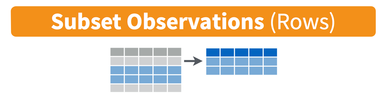
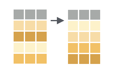
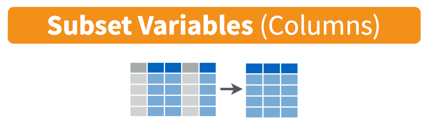
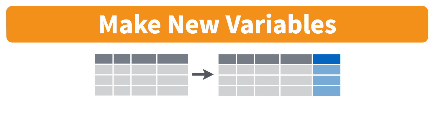
• filter() picks out rows according to specified conditions
• arrange() sorts the row by values in some column(s)
• select() picks out columns according to their names
• mutate() creates new columns, often based on operations on other columns

All work similarly:

1. The first argument is a data frame.
2. The subsequent arguments describe what to do with the data frame, using the variable names (without quotes).
3. The result is a new data frame.

Together these properties make it easy to chain together multiple simple steps to achieve a complex result.

Later we will also learn

• summarize() collapses many values in one or more columns down to one value per column

and group_by() which changes the scope of each function from operating on the entire dataset to operating on it group-by-group.

GTEx data

This is a subset of the Genotype Tissue Expression (GTEx) dataset

• The full dataset. Includes gene expression data, measured via RNA-sequencing, from 54 post-mortem tissues in ~800 individuals. Whole genome sequencing is also available for these individuals as part of the GTEx v8 release, available through dbGaP.
• The subsetted dataset. We are looking at expression data for just 78 individuals here, in four tissues including blood, heart, lung and liver.
• Data processing The expression values have been normalized and corrected for technical covariates and are now in the form of “Z-scores”, which indicate the distance of a given expression value from the mean across all measurements of that gene in that tissue.
• Goal. We will use the data here to illustrate different functions for data transformation, often focused on extracting individuals with extremely high or low expression values for a given gene as compared to the distribution across all samples.

# Read subsetted data from online file - make sure there are no spaces
gtex = read_tsv('https://tinyurl.com/342rhdc2')

# Check number of rows
nrow(gtex)

[1] 389922

Filter rows with filter()

Filter rows with filter()

• filter() lets you filter out rows of a dataset that meet a certain condition

• filter() lets you filter out rows of a dataset that meet a certain condition
• It takes two arguments: the dataset and the condition

filter(gtex, Blood >= 12)

# A tibble: 12 × 6
   Gene       Ind        Blood Heart  Lung Liver
   <chr>      <chr>      <dbl> <dbl> <dbl> <dbl>
 1 AC012358.7 GTEX-VUSG   13.6 -1.43  1.22 -0.39
 2 DCSTAMP    GTEX-12696  13.6 NA    -0.57 -0.91
 3 DIAPH2-AS1 GTEX-VUSG   12.2 -0.33  1.18  0.67
 4 DNASE2B    GTEX-12696  14.4 -0.82 -0.92  0.35
 5 FFAR4      GTEX-12696  12.9 -0.96 -0.67  0.18
 6 GAPDHP33   GTEX-UPK5   13.8  1.52 -1.48 -1.84
 7 GTF2A1L    GTEX-VUSG   12.2  1.67  0.78  0.09
 8 GTF2IP14   GTEX-11NV4  12.2  7.26  5.79  7.06
 9 KCNT1      GTEX-1KANB  13.5  3.14  0.62 -0.37
10 KLK3       GTEX-147F4  15.7 -0.74 -0.44 -0.02
11 NAPSA      GTEX-1CB4J  12.3 -0.29 -0.44 -0.14
12 REN        GTEX-U8XE   18.9 -0.57 NA     0.09

Comparisons

• == and != test for equality and inequality (do not use = for equality)
• > and < test for greater-than and less-than
• >= and <= are greater-than-or-equal and less-than-or-equal
• these can also be used directly on vectors outside of data frames

c(1,5,-22,4) > 0

[1]  TRUE  TRUE FALSE  TRUE

c("a", "b", "c") == "b"

[1] FALSE  TRUE FALSE

Comparing to NA

• A common “gotcha” is that == cannot be used to compare to NA:

x = NA
x == NA

[1] NA

• The result actually makes sense though, because I’m asking if “I don’t know” is the same as “I don’t know”. Since either side could be any value, the right answer is “I don’t know”.
• To check if something is NA, use is.na()

x = NA
is.na(x)

[1] TRUE

Equality on Strings

• you can use == to test whether a string variable matches given text
• but remember to quote the text you want to compare to

filter(gtex, Gene == "ZZZ3")

# A tibble: 78 × 6
   Gene  Ind        Blood Heart  Lung Liver
   <chr> <chr>      <dbl> <dbl> <dbl> <dbl>
 1 ZZZ3  GTEX-11DXZ  1.37 -0.06  1.74  0.41
 2 ZZZ3  GTEX-11GSP -0.68 -1.83  0.8   0.93
 3 ZZZ3  GTEX-11NUK -0.75 -3.41  0.73  0.39
 4 ZZZ3  GTEX-11NV4  0.6  -0.28 -0.23 -0.05
 5 ZZZ3  GTEX-11TT1  0.86  0.93  0.07  1.3 
 6 ZZZ3  GTEX-11TUW  0.15  0.68 -0.43  1.23
 7 ZZZ3  GTEX-11ZUS -2.29 -0.78 NA     0.6 
 8 ZZZ3  GTEX-11ZVC -0.98 -1.4   1.22 -1.32
 9 ZZZ3  GTEX-1212Z -0.36 -0.33 -0.34  0.57
10 ZZZ3  GTEX-12696 -1.37 -0.9   1.03  0.22
# ℹ 68 more rows

• why doesn’t Gene == ZZZ3 work?
• why doesn’t "Gene" == "ZZZ3" make sense?

Filtering on computed values

• the condition can contain computed values

filter(gtex, Blood + Heart > 0)

# A tibble: 185,944 × 6
   Gene  Ind        Blood Heart  Lung Liver
   <chr> <chr>      <dbl> <dbl> <dbl> <dbl>
 1 A2ML1 GTEX-11GSP -0.5   0.53  0.76 -0.1 
 2 A2ML1 GTEX-1212Z -0.3   0.53  0.1  -0.48
 3 A2ML1 GTEX-12696 -0.11  0.24  0.96  0.72
 4 A2ML1 GTEX-12WSD  0.53  0.36  0.2   0.51
 5 A2ML1 GTEX-12WSI  0     0.2  -0.21 -0.07
 6 A2ML1 GTEX-131XE  0.3   0.05  0.53 -0.87
 7 A2ML1 GTEX-132NY  0.42 -0.14 -0.27  1.47
 8 A2ML1 GTEX-13FTZ -0.11  1.12  0.49  1.43
 9 A2ML1 GTEX-13OW6  0.15 -0.13  1.06  0.24
10 A2ML1 GTEX-14DAQ  0.1   0.69  0.99 -0.79
# ℹ 185,934 more rows

• note that we didn’t actually do anything to the values in the data

Exercise [together]

• What is the result of running this code?

nrow(gtex)

[1] 389922

filter(gtex, Gene == "ZZZ3")
filter(gtex, Heart <= -5)
nrow(gtex)

Exercise

• Without using the internet, think of how you can use filter multiple times to create a dataset where blood expression is positive (>0) and heart expression is negative (<0)

• Using any resources you like, figure out how to use filter to create a dataset where either blood expression is positive (>0) or heart expression is negative (<0)

Logical conjunctions (AND)

filter(gtex, Blood < 0 & Heart < 0)

# A tibble: 104,686 × 6
   Gene  Ind        Blood Heart  Lung Liver
   <chr> <chr>      <dbl> <dbl> <dbl> <dbl>
 1 A2ML1 GTEX-11DXZ -0.14 -1.08 NA    -0.66
 2 A2ML1 GTEX-11NUK -0.08 -0.4  -0.26 -0.13
 3 A2ML1 GTEX-11ZUS -1.07 -0.41  0.67  0.06
 4 A2ML1 GTEX-11ZVC -0.27 -0.51  0.13 -0.75
 5 A2ML1 GTEX-14BIL -0.32 -1.3   0.39 -0.58
 6 A2ML1 GTEX-14JG1 -0.59 -0.61 -0.36 -1.94
 7 A2ML1 GTEX-14PJO -0.07 -0.96  1.27  0.48
 8 A2ML1 GTEX-17EVP -1    -0.18 -0.2  -0.95
 9 A2ML1 GTEX-18465 -0.38 -0.4   0.1   0.5 
10 A2ML1 GTEX-18A7A -1.01 -0.74 -0.72 -0.76
# ℹ 104,676 more rows

• This filters by the conjunction of the two constraints—both must be satisfied.
• The ampersand sign & stands for “AND”

TRUE & FALSE

[1] FALSE

TRUE & TRUE

[1] TRUE

FALSE & TRUE

[1] FALSE

• For filter, you can do “AND” by passing in two separate conditions as two different arguments, but the comma and ampersand are not generally interchangeable

# filter(gtex, Blood < 0 & Heart < 0)
filter(gtex, Blood < 0, Heart < 0)

# A tibble: 104,686 × 6
   Gene  Ind        Blood Heart  Lung Liver
   <chr> <chr>      <dbl> <dbl> <dbl> <dbl>
 1 A2ML1 GTEX-11DXZ -0.14 -1.08 NA    -0.66
 2 A2ML1 GTEX-11NUK -0.08 -0.4  -0.26 -0.13
 3 A2ML1 GTEX-11ZUS -1.07 -0.41  0.67  0.06
 4 A2ML1 GTEX-11ZVC -0.27 -0.51  0.13 -0.75
 5 A2ML1 GTEX-14BIL -0.32 -1.3   0.39 -0.58
 6 A2ML1 GTEX-14JG1 -0.59 -0.61 -0.36 -1.94
 7 A2ML1 GTEX-14PJO -0.07 -0.96  1.27  0.48
 8 A2ML1 GTEX-17EVP -1    -0.18 -0.2  -0.95
 9 A2ML1 GTEX-18465 -0.38 -0.4   0.1   0.5 
10 A2ML1 GTEX-18A7A -1.01 -0.74 -0.72 -0.76
# ℹ 104,676 more rows

Logical conjunctions (OR)

filter(gtex, Gene == "A2ML1" | Gene == "A4GALT")

# A tibble: 156 × 6
   Gene  Ind        Blood Heart  Lung Liver
   <chr> <chr>      <dbl> <dbl> <dbl> <dbl>
 1 A2ML1 GTEX-11DXZ -0.14 -1.08 NA    -0.66
 2 A2ML1 GTEX-11GSP -0.5   0.53  0.76 -0.1 
 3 A2ML1 GTEX-11NUK -0.08 -0.4  -0.26 -0.13
 4 A2ML1 GTEX-11NV4 -0.37  0.11 -0.42 -0.61
 5 A2ML1 GTEX-11TT1  0.3  -1.11  0.59 -0.12
 6 A2ML1 GTEX-11TUW  0.02 -0.47  0.29 -0.66
 7 A2ML1 GTEX-11ZUS -1.07 -0.41  0.67  0.06
 8 A2ML1 GTEX-11ZVC -0.27 -0.51  0.13 -0.75
 9 A2ML1 GTEX-1212Z -0.3   0.53  0.1  -0.48
10 A2ML1 GTEX-12696 -0.11  0.24  0.96  0.72
# ℹ 146 more rows

• The pipe sign | stands for “OR”
• Multiple conjunctions can describe complex logical conditions

filter(gtex, Gene %in% c("ZZZ3","A2ML1")) 

# A tibble: 156 × 6
   Gene  Ind        Blood Heart  Lung Liver
   <chr> <chr>      <dbl> <dbl> <dbl> <dbl>
 1 A2ML1 GTEX-11DXZ -0.14 -1.08 NA    -0.66
 2 A2ML1 GTEX-11GSP -0.5   0.53  0.76 -0.1 
 3 A2ML1 GTEX-11NUK -0.08 -0.4  -0.26 -0.13
 4 A2ML1 GTEX-11NV4 -0.37  0.11 -0.42 -0.61
 5 A2ML1 GTEX-11TT1  0.3  -1.11  0.59 -0.12
 6 A2ML1 GTEX-11TUW  0.02 -0.47  0.29 -0.66
 7 A2ML1 GTEX-11ZUS -1.07 -0.41  0.67  0.06
 8 A2ML1 GTEX-11ZVC -0.27 -0.51  0.13 -0.75
 9 A2ML1 GTEX-1212Z -0.3   0.53  0.1  -0.48
10 A2ML1 GTEX-12696 -0.11  0.24  0.96  0.72
# ℹ 146 more rows

# equivalent to 
# filter(gtex, Gene=="ZZZ3" | Gene=="A2ML1")

• %in% returns true for all elements of the thing on the left that are also elements of the thing on the right. This is actually shorthand for a match function (use help('%in%') to learn more)

Negation (NOT)

filter(gtex, !(Gene=="A2ML1"))

# A tibble: 389,844 × 6
   Gene    Ind        Blood Heart  Lung Liver
   <chr>   <chr>      <dbl> <dbl> <dbl> <dbl>
 1 A3GALT2 GTEX-11DXZ -0.48 -1     1.83 -0.4 
 2 A3GALT2 GTEX-11GSP -0.39  2.09  0.88 -0.78
 3 A3GALT2 GTEX-11NUK -0.36 -0.27 NA     0.2 
 4 A3GALT2 GTEX-11NV4 -0.77 -0.08  0.13  0.06
 5 A3GALT2 GTEX-11TT1 -1.4   1.29  1.45  1.57
 6 A3GALT2 GTEX-11TUW  0.15 -3.41  0.96 -0.83
 7 A3GALT2 GTEX-11ZUS -0.03 -0.32  0.25 -0.73
 8 A3GALT2 GTEX-11ZVC -0.21 -0.75  0.59 -0.66
 9 A3GALT2 GTEX-1212Z  0.36 -0.12  0.78  1.5 
10 A3GALT2 GTEX-12696 -0.25 -0.31 -0.03  2.62
# ℹ 389,834 more rows

• The exclamation point ! means “NOT”, which negates the logical condition
• sometimes it’s easier to say what you don’t want!

Exercises: computed conditions, conjunctions, NAs

Do each of these three exercises separately

• Filter the GTEX data to keep just the rows where the product of Blood and Heart expression is between 0 and 1.

• Excluding the gene LAMP3, does the individual GTEX-11TT1 have any genes with expression level greater than 4 in their blood?

• Filter out any rows where the value for Heart is missing (value is NA)

Sampling rows

• You can use slice_sample() to get n randomly selected rows if you don’t have a particular condition you would like to filter on.

slice_sample(gtex, n=5)

# A tibble: 5 × 6
  Gene        Ind        Blood Heart  Lung Liver
  <chr>       <chr>      <dbl> <dbl> <dbl> <dbl>
1 RP11-11N9.4 GTEX-14PJO -0.43  1.08 -1.06  0.08
2 LRRC37A3    GTEX-147F4 -0.06 -1.97 -1.77 -0.3 
3 ZMYND11     GTEX-ZAB4  -0.84  0.7   1.6   1   
4 COX6B2      GTEX-1KANB  0.65 -0.71  0.64  1.39
5 CD58        GTEX-11ZUS  1.51 -0.32  0.78 -0.16

• the named argument prop allows you to sample a proportion of rows
• Do ?slice_sample() to see how you can sample with replacement or with weights

Filtering by row number

• Data frames typically don’t have a row_number column that you can reference, but you can invisibly create one for filter to operate on with row_number()
• This is more useful once you have sorted the data in a particular order, which we will soon see how to do.

filter(gtex, row_number()<=3)

# A tibble: 3 × 6
  Gene  Ind        Blood Heart  Lung Liver
  <chr> <chr>      <dbl> <dbl> <dbl> <dbl>
1 A2ML1 GTEX-11DXZ -0.14 -1.08 NA    -0.66
2 A2ML1 GTEX-11GSP -0.5   0.53  0.76 -0.1 
3 A2ML1 GTEX-11NUK -0.08 -0.4  -0.26 -0.13

Sort rows with arrange()

Sort rows with arrange()

• arrange() takes a data frame and a column, and sorts the rows by the values in that column (ascending order).

• arrange() takes a data frame and a column, and sorts the rows by the values in that column (ascending order).
• Again, the first argument is the data frame and the other arguments tell the function what to do with it

arrange(gtex, Blood)

# A tibble: 389,922 × 6
   Gene        Ind        Blood  Heart   Lung Liver
   <chr>       <chr>      <dbl>  <dbl>  <dbl> <dbl>
 1 HBA2        GTEX-11DXZ -9.44  -1.52  -1.44 -2.15
 2 MTATP6P1    GTEX-1KD5A -9.18 -10.1  -10.3  -9.52
 3 RP11-46D6.1 GTEX-14E1K -7.83  -3.94  -5.22 -4.49
 4 CYTH3       GTEX-11NV4 -6.63  -0.6   -0.37 -1.32
 5 TRG-AS1     GTEX-11NV4 -6.47   2.39  -0.6  -0.22
 6 SMG1P1      GTEX-11ZUS -6.26  -1.68  -1.41 -0.31
 7 ZBTB10      GTEX-VUSG  -6.13   0.77   0.51 -0.67
 8 RPS29       GTEX-1B8L1 -5.84  -0.8   -0.46 -0.17
 9 GHITM       GTEX-WK11  -5.7   -7.24  -7.37 -4.06
10 ZNF2        GTEX-VUSG  -5.62   1.52   0.61  0.13
# ℹ 389,912 more rows

Descending sort

• Use the desc function to arrange by descending values

arrange(gtex, desc(Blood))

# A tibble: 389,922 × 6
   Gene       Ind        Blood Heart  Lung Liver
   <chr>      <chr>      <dbl> <dbl> <dbl> <dbl>
 1 REN        GTEX-U8XE   18.9 -0.57 NA     0.09
 2 KLK3       GTEX-147F4  15.7 -0.74 -0.44 -0.02
 3 DNASE2B    GTEX-12696  14.4 -0.82 -0.92  0.35
 4 GAPDHP33   GTEX-UPK5   13.8  1.52 -1.48 -1.84
 5 DCSTAMP    GTEX-12696  13.6 NA    -0.57 -0.91
 6 AC012358.7 GTEX-VUSG   13.6 -1.43  1.22 -0.39
 7 KCNT1      GTEX-1KANB  13.5  3.14  0.62 -0.37
 8 FFAR4      GTEX-12696  12.9 -0.96 -0.67  0.18
 9 NAPSA      GTEX-1CB4J  12.3 -0.29 -0.44 -0.14
10 DIAPH2-AS1 GTEX-VUSG   12.2 -0.33  1.18  0.67
# ℹ 389,912 more rows

Multisort

• This is useful if there is a tie in sorting by the first column.

arrange(gtex, Gene, Blood)

# A tibble: 389,922 × 6
   Gene  Ind        Blood Heart  Lung Liver
   <chr> <chr>      <dbl> <dbl> <dbl> <dbl>
 1 A2ML1 GTEX-1B8L1 -1.4   0.37 -1.05  0.07
 2 A2ML1 GTEX-ZVT3  -1.35  1.01  2.91 -0.28
 3 A2ML1 GTEX-1AX9I -1.29 -0.19 -0.41 -0.78
 4 A2ML1 GTEX-1A32A -1.16  0.44 -0.41 -0.39
 5 A2ML1 GTEX-1GN73 -1.13 -0.05 -0.21 -0.82
 6 A2ML1 GTEX-11ZUS -1.07 -0.41  0.67  0.06
 7 A2ML1 GTEX-18A7A -1.01 -0.74 -0.72 -0.76
 8 A2ML1 GTEX-17EVP -1    -0.18 -0.2  -0.95
 9 A2ML1 GTEX-U8XE  -0.88 -0.91 NA    -0.86
10 A2ML1 GTEX-131YS -0.78 NA     0.17 -1.5 
# ℹ 389,912 more rows

Exercise: top 5 high expression instances

Use arrange() and filter() to get the data for the 5 rows with the highest expression values in blood

Piping

Nesting and Temporary Variables

• In our last exercise, we used two function applications to arrive at our answer. Shown below, we used temporary variables to keep our code clean.

gtex_by_blood = arrange(gtex, desc(Blood)) # using a temporary variable
filter(gtex_by_blood, row_number()<=5)

# A tibble: 5 × 6
  Gene     Ind        Blood Heart  Lung Liver
  <chr>    <chr>      <dbl> <dbl> <dbl> <dbl>
1 REN      GTEX-U8XE   18.9 -0.57 NA     0.09
2 KLK3     GTEX-147F4  15.7 -0.74 -0.44 -0.02
3 DNASE2B  GTEX-12696  14.4 -0.82 -0.92  0.35
4 GAPDHP33 GTEX-UPK5   13.8  1.52 -1.48 -1.84
5 DCSTAMP  GTEX-12696  13.6 NA    -0.57 -0.91

• we can also accompish this by “nesting” the function calls:

filter(arrange(gtex, desc(Blood)), row_number()<=5) # "nesting" the calls to filter and arrange

# A tibble: 5 × 6
  Gene     Ind        Blood Heart  Lung Liver
  <chr>    <chr>      <dbl> <dbl> <dbl> <dbl>
1 REN      GTEX-U8XE   18.9 -0.57 NA     0.09
2 KLK3     GTEX-147F4  15.7 -0.74 -0.44 -0.02
3 DNASE2B  GTEX-12696  14.4 -0.82 -0.92  0.35
4 GAPDHP33 GTEX-UPK5   13.8  1.52 -1.48 -1.84
5 DCSTAMP  GTEX-12696  13.6 NA    -0.57 -0.91

• Which do you prefer? Why? What are the sylistic pros and cons to both if you are trying to understand what the code does for the first time?

The pipe

• R solves these problems with the “pipe” operator |>

gtex |> 
  arrange(desc(Blood)) |>
  filter(row_number()<=5)

• How does this compare with our code before? What do you notice?

gtex_by_blood = arrange(gtex, desc(Blood)) # using a temporary variable
filter(gtex_by_blood, row_number()<=5)

Pipe syntax

When df1 is piped into fun(x) (fun is just some fake function)

df1 |> fun(x)

is converted into:

fun(df1, x)

• That is: the thing being piped in is used as the first argument of fun.
• The tidyverse functions are consistently designed so that the first argument is a data frame, and the result is a data frame, so you can push a dataframe all the way through a series of functions

• The pipe represents a “conveyor belt” along which data is passed from function to function (“workers”) in an assembly line

gtex |> 
  arrange(desc(Blood)) |>
  filter(row_number()<=5)

# same as:
#   arrange(gtex, desc(Blood)) |>
#   filter(row_number()<=5)


# same as:
#   filter( arrange(gtex, desc(Blood)), row_number()<=5)

• The pipe works for all variables and functions (not just tidyverse functions)

Piping a string

# paste("hello", "world")
"hello" |> paste("world") 

[1] "hello world"

Piping a vector

# sum(c(1,44,21,0,-4))
c(1,44,21,0,-4) |> sum()

[1] 62

Piping a data frame

# filter(gtex, Gene=="ZZZ3")
gtex |> filter(Gene=="ZZZ3") 

# A tibble: 78 × 6
   Gene  Ind        Blood Heart  Lung Liver
   <chr> <chr>      <dbl> <dbl> <dbl> <dbl>
 1 ZZZ3  GTEX-11DXZ  1.37 -0.06  1.74  0.41
 2 ZZZ3  GTEX-11GSP -0.68 -1.83  0.8   0.93
 3 ZZZ3  GTEX-11NUK -0.75 -3.41  0.73  0.39
 4 ZZZ3  GTEX-11NV4  0.6  -0.28 -0.23 -0.05
 5 ZZZ3  GTEX-11TT1  0.86  0.93  0.07  1.3 
 6 ZZZ3  GTEX-11TUW  0.15  0.68 -0.43  1.23
 7 ZZZ3  GTEX-11ZUS -2.29 -0.78 NA     0.6 
 8 ZZZ3  GTEX-11ZVC -0.98 -1.4   1.22 -1.32
 9 ZZZ3  GTEX-1212Z -0.36 -0.33 -0.34  0.57
10 ZZZ3  GTEX-12696 -1.37 -0.9   1.03  0.22
# ℹ 68 more rows

Two Pipes

History - R had no pipe - ~2014: introduced by magrittr package (as %>%) - ~2016: tidyverse adoption, proliferated in code - ~2021: base language adopted idea, implemented native pipe |>

• %>% and |> are (basically) the same
• you will see both in the wild

filter(gtex, Gene=="ZZZ3")
gtex |> filter(Gene=="ZZZ3") 
gtex %>% filter(Gene=="ZZZ3") 

Exercise: Pipe to ggplot

• Run this code to see what it does. Then rewrite it using the pipe operator (get rid of the intermediate variables mybl2 and outliers) and get it to produce the same output.

mybl2 = filter(gtex, Gene == 'MYBL2')

# we haven't learned about this function yet, but doesn't matter
outliers = mutate(mybl2, blood_outlier = abs(Blood) > 2) 

ggplot(outliers) +
  geom_bar(aes(x=blood_outlier))

Select columns with select()

Select columns with select()

• The select function will return a subset of the tibble, using only the requested columns in the order specified.

• The select function will return a subset of the tibble, using only the requested columns in the order specified.
• first argument is a data frame, then columns you want to select

gtex |>
  select(Gene, Ind, expression=Blood)

# A tibble: 389,922 × 3
   Gene  Ind        expression
   <chr> <chr>           <dbl>
 1 A2ML1 GTEX-11DXZ      -0.14
 2 A2ML1 GTEX-11GSP      -0.5 
 3 A2ML1 GTEX-11NUK      -0.08
 4 A2ML1 GTEX-11NV4      -0.37
 5 A2ML1 GTEX-11TT1       0.3 
 6 A2ML1 GTEX-11TUW       0.02
 7 A2ML1 GTEX-11ZUS      -1.07
 8 A2ML1 GTEX-11ZVC      -0.27
 9 A2ML1 GTEX-1212Z      -0.3 
10 A2ML1 GTEX-12696      -0.11
# ℹ 389,912 more rows

• you can rename columns in the result with the syntax new_name = old_name

Helpers

• select() can also be used with handy helpers like starts_with() and contains()

gtex |>
  select(starts_with("L"))

# A tibble: 389,922 × 2
    Lung Liver
   <dbl> <dbl>
 1 NA    -0.66
 2  0.76 -0.1 
 3 -0.26 -0.13
 4 -0.42 -0.61
 5  0.59 -0.12
 6  0.29 -0.66
 7  0.67  0.06
 8  0.13 -0.75
 9  0.1  -0.48
10  0.96  0.72
# ℹ 389,912 more rows

• Use ?select to see all the possibilities

gtex |>
  select(contains("N"))

# A tibble: 389,922 × 3
   Gene  Ind         Lung
   <chr> <chr>      <dbl>
 1 A2ML1 GTEX-11DXZ NA   
 2 A2ML1 GTEX-11GSP  0.76
 3 A2ML1 GTEX-11NUK -0.26
 4 A2ML1 GTEX-11NV4 -0.42
 5 A2ML1 GTEX-11TT1  0.59
 6 A2ML1 GTEX-11TUW  0.29
 7 A2ML1 GTEX-11ZUS  0.67
 8 A2ML1 GTEX-11ZVC  0.13
 9 A2ML1 GTEX-1212Z  0.1 
10 A2ML1 GTEX-12696  0.96
# ℹ 389,912 more rows

• The quotes around the letter "N" make it a string. If we did not do this, R would think it was looking for a variable called N and not just the plain letter.
• We don’t have to quote the names of columns (like Ind) because the tidyverse functions know that we are working within the dataframe and thus treat the column names like they are variables in their own right

• we can even select columns based on metadata (but not values!)

gtex |>
  select(where(is.numeric))

# A tibble: 389,922 × 4
   Blood Heart  Lung Liver
   <dbl> <dbl> <dbl> <dbl>
 1 -0.14 -1.08 NA    -0.66
 2 -0.5   0.53  0.76 -0.1 
 3 -0.08 -0.4  -0.26 -0.13
 4 -0.37  0.11 -0.42 -0.61
 5  0.3  -1.11  0.59 -0.12
 6  0.02 -0.47  0.29 -0.66
 7 -1.07 -0.41  0.67  0.06
 8 -0.27 -0.51  0.13 -0.75
 9 -0.3   0.53  0.1  -0.48
10 -0.11  0.24  0.96  0.72
# ℹ 389,912 more rows

Negation

• select() can also be used to select everything except for certain columns

gtex |>
  select(-starts_with("L"), -Ind)

# A tibble: 389,922 × 3
   Gene  Blood Heart
   <chr> <dbl> <dbl>
 1 A2ML1 -0.14 -1.08
 2 A2ML1 -0.5   0.53
 3 A2ML1 -0.08 -0.4 
 4 A2ML1 -0.37  0.11
 5 A2ML1  0.3  -1.11
 6 A2ML1  0.02 -0.47
 7 A2ML1 -1.07 -0.41
 8 A2ML1 -0.27 -0.51
 9 A2ML1 -0.3   0.53
10 A2ML1 -0.11  0.24
# ℹ 389,912 more rows

Exercise: select and filter

A colleague wants to see the blood expression for the gene A2ML1 for each person. Use select and filter to produce a dataframe for her that has just two columns: individual and expression, where the expression values are the blood expression values for each person for the gene A2ML1.

Before writing any code, break the problem down conceptually into steps. Figure out how to do each step independently before you put them together.

pull()

• select() has a friend called pull() which returns a vector instead of a (one-column) data frame

gtex |> pull(Gene)

 [1] "A2ML1" "A2ML1" "A2ML1" "A2ML1" "A2ML1" "A2ML1" "A2ML1" "A2ML1" "A2ML1"
[10] "A2ML1"

gtex |> select(Gene)

# A tibble: 10 × 1
   Gene 
   <chr>
 1 A2ML1
 2 A2ML1
 3 A2ML1
 4 A2ML1
 5 A2ML1
 6 A2ML1
 7 A2ML1
 8 A2ML1
 9 A2ML1
10 A2ML1

Rename columns

• select() can be used to rename variables, but it drops all variables not selected

gtex |> select(individual = Ind)

# A tibble: 389,922 × 1
   individual
   <chr>     
 1 GTEX-11DXZ
 2 GTEX-11GSP
 3 GTEX-11NUK
 4 GTEX-11NV4
 5 GTEX-11TT1
 6 GTEX-11TUW
 7 GTEX-11ZUS
 8 GTEX-11ZVC
 9 GTEX-1212Z
10 GTEX-12696
# ℹ 389,912 more rows

• rename() is better suited for this because it keeps all the columns

gtex |> rename(individual = Ind)

# A tibble: 389,922 × 6
   Gene  individual Blood Heart  Lung Liver
   <chr> <chr>      <dbl> <dbl> <dbl> <dbl>
 1 A2ML1 GTEX-11DXZ -0.14 -1.08 NA    -0.66
 2 A2ML1 GTEX-11GSP -0.5   0.53  0.76 -0.1 
 3 A2ML1 GTEX-11NUK -0.08 -0.4  -0.26 -0.13
 4 A2ML1 GTEX-11NV4 -0.37  0.11 -0.42 -0.61
 5 A2ML1 GTEX-11TT1  0.3  -1.11  0.59 -0.12
 6 A2ML1 GTEX-11TUW  0.02 -0.47  0.29 -0.66
 7 A2ML1 GTEX-11ZUS -1.07 -0.41  0.67  0.06
 8 A2ML1 GTEX-11ZVC -0.27 -0.51  0.13 -0.75
 9 A2ML1 GTEX-1212Z -0.3   0.53  0.1  -0.48
10 A2ML1 GTEX-12696 -0.11  0.24  0.96  0.72
# ℹ 389,912 more rows

Add new variables with mutate()

Add new variables with mutate()

• mutate creates new columns

• mutate creates new columns
• first argument is a dataframe, second specifies what you want the new columns to be

gtex |>
  mutate(scaled_blood = 100*Blood))

Error: <text>:2:35: unexpected ')'
1: gtex |>
2:   mutate(scaled_blood = 100*Blood))
                                     ^

• This uses mutate() to add a new column to which is the absolute value of Blood.
• The thing on the left of the = is a new name that you make up which you would like the new column to be called
• The expression on the right of the = defines what will go into the new column

• Warning! If the new variable name already exists, mutate() will overwrite the existing one (in the new dataframe that gets created)

gtex |>
  mutate(Blood = 100*Blood)

# A tibble: 389,922 × 6
   Gene  Ind        Blood Heart  Lung Liver
   <chr> <chr>      <dbl> <dbl> <dbl> <dbl>
 1 A2ML1 GTEX-11DXZ   -14 -1.08 NA    -0.66
 2 A2ML1 GTEX-11GSP   -50  0.53  0.76 -0.1 
 3 A2ML1 GTEX-11NUK    -8 -0.4  -0.26 -0.13
 4 A2ML1 GTEX-11NV4   -37  0.11 -0.42 -0.61
 5 A2ML1 GTEX-11TT1    30 -1.11  0.59 -0.12
 6 A2ML1 GTEX-11TUW     2 -0.47  0.29 -0.66
 7 A2ML1 GTEX-11ZUS  -107 -0.41  0.67  0.06
 8 A2ML1 GTEX-11ZVC   -27 -0.51  0.13 -0.75
 9 A2ML1 GTEX-1212Z   -30  0.53  0.1  -0.48
10 A2ML1 GTEX-12696   -11  0.24  0.96  0.72
# ℹ 389,912 more rows

• mutate() can create multiple columns at the same time and use multiple columns to define a single new one

gtex |>
  mutate(  # the newlines make it more readable
      scaled_blood = 100* Blood,
      scaled_heart = 100* Heart,
      scaled_blood_heart_dif = scaled_blood - scaled_heart
  )

# A tibble: 389,922 × 9
   Gene  Ind        Blood Heart  Lung Liver scaled_blood scaled_heart
   <chr> <chr>      <dbl> <dbl> <dbl> <dbl>        <dbl>        <dbl>
 1 A2ML1 GTEX-11DXZ -0.14 -1.08 NA    -0.66          -14         -108
 2 A2ML1 GTEX-11GSP -0.5   0.53  0.76 -0.1           -50           53
 3 A2ML1 GTEX-11NUK -0.08 -0.4  -0.26 -0.13           -8          -40
 4 A2ML1 GTEX-11NV4 -0.37  0.11 -0.42 -0.61          -37           11
 5 A2ML1 GTEX-11TT1  0.3  -1.11  0.59 -0.12           30         -111
 6 A2ML1 GTEX-11TUW  0.02 -0.47  0.29 -0.66            2          -47
 7 A2ML1 GTEX-11ZUS -1.07 -0.41  0.67  0.06         -107          -41
 8 A2ML1 GTEX-11ZVC -0.27 -0.51  0.13 -0.75          -27          -51
 9 A2ML1 GTEX-1212Z -0.3   0.53  0.1  -0.48          -30           53
10 A2ML1 GTEX-12696 -0.11  0.24  0.96  0.72          -11           24
# ℹ 389,912 more rows
# ℹ 1 more variable: scaled_blood_heart_dif <dbl>

• Note that we have also used two columns simultaneously to create a new column

• mutate is used for text data too

library(stringr)

gtex |>
  mutate(Ind_ID_suffix = str_extract(Ind, "(GTEX-)(.*)", group=2)) |>
  select(Ind, Ind_ID_suffix)

# A tibble: 389,922 × 2
   Ind        Ind_ID_suffix
   <chr>      <chr>        
 1 GTEX-11DXZ 11DXZ        
 2 GTEX-11GSP 11GSP        
 3 GTEX-11NUK 11NUK        
 4 GTEX-11NV4 11NV4        
 5 GTEX-11TT1 11TT1        
 6 GTEX-11TUW 11TUW        
 7 GTEX-11ZUS 11ZUS        
 8 GTEX-11ZVC 11ZVC        
 9 GTEX-1212Z 1212Z        
10 GTEX-12696 12696        
# ℹ 389,912 more rows

Type conversion

• Data is sometimes given to you in a form that makes it difficult to do operations on

df = tibble(number = c("1", "2", "3"))
df

# A tibble: 3 × 1
  number
  <chr> 
1 1     
2 2     
3 3     

df |> mutate(number_plus_1 = number + 1)

Error in `mutate()`:
ℹ In argument: `number_plus_1 = number + 1`.
Caused by error in `number + 1`:
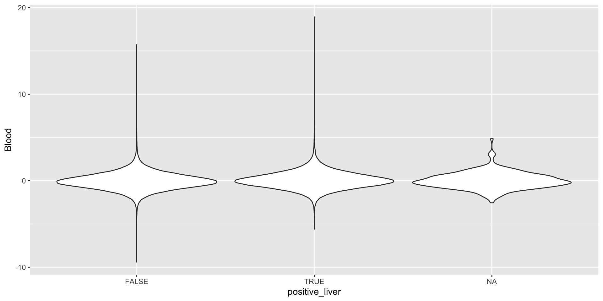
! non-numeric argument to binary operator

• mutate() is also useful for converting data types, in this case text to numbers

df |> mutate(number = as.numeric(number))

# A tibble: 3 × 1
  number
   <dbl>
1      1
2      2
3      3

Indicators

• mutate() can be used to make logical columns (indicators)

gtex |>
  mutate(positive_liver = Liver > 0) |>
  select(Gene, Ind, Liver, positive_liver)

# A tibble: 389,922 × 4
   Gene  Ind        Liver positive_liver
   <chr> <chr>      <dbl> <lgl>         
 1 A2ML1 GTEX-11DXZ -0.66 FALSE         
 2 A2ML1 GTEX-11GSP -0.1  FALSE         
 3 A2ML1 GTEX-11NUK -0.13 FALSE         
 4 A2ML1 GTEX-11NV4 -0.61 FALSE         
 5 A2ML1 GTEX-11TT1 -0.12 FALSE         
 6 A2ML1 GTEX-11TUW -0.66 FALSE         
 7 A2ML1 GTEX-11ZUS  0.06 TRUE          
 8 A2ML1 GTEX-11ZVC -0.75 FALSE         
 9 A2ML1 GTEX-1212Z -0.48 FALSE         
10 A2ML1 GTEX-12696  0.72 TRUE          
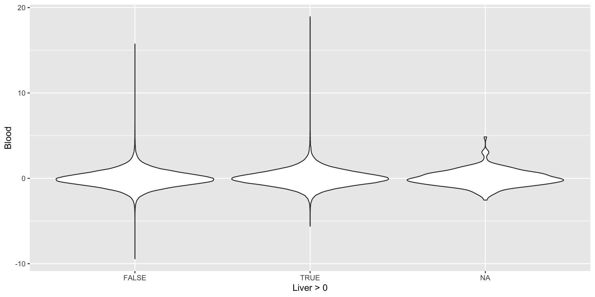
# ℹ 389,912 more rows

• which can be used to make plots

gtex |>
  mutate(positive_liver = Liver > 0) |>
ggplot(aes(x=positive_liver, y=Blood)) +
  geom_violin()

or you can just “mutate” directly in ggplot!

gtex |>  # mutate(positive_liver = Liver > 0) |>
ggplot(aes(x=Liver > 0, y=Blood)) +
  geom_violin()

Exercise: mutate()

Before writing code for each problem , break the problem into steps. Do you have to create new columns? Filter rows? Arrange rows? Select columns? In what order? Once you have a plan, write code, one step at a time.

Problem 1

I want to see if certain genes are generally more highly expressed in certain individuals, irrespective of tissue type. Using the GTEX data, create a new column containing the sum of the four expression measurements in the different tissues.

Problem 2

Produce a plot showing blood vs heart expression of the MYL1 gene only and assign color based on positive vs. negative expression of that gene in liver tissue.

Problem 3

Produce a vector containing the ten individual IDs (Ind) with the biggest difference in their heart and lung expression for the A2ML1 gene.

mutate() and if_else()

• if_else is a vectorized if-else statement
• the first argument is an R expression that evaluates to a logical vector, the second argument is what to replace all of the resulting TRUEs with, and the third argument is what to replace the resulting FALSEs with

x = c(-1, 1/2, 2/3, 5)
if_else(0<=x & x<=1, "in [0,1]", "not in [0,1]")

[1] "not in [0,1]" "in [0,1]"     "in [0,1]"     "not in [0,1]"

• this is often used in mutate():

gtex |>
mutate( 
  blood_expression = ifelse(
    Blood < 0, "-", "+"
))

# A tibble: 389,922 × 7
   Gene  Ind        Blood Heart  Lung Liver blood_expression
   <chr> <chr>      <dbl> <dbl> <dbl> <dbl> <chr>           
 1 A2ML1 GTEX-11DXZ -0.14 -1.08 NA    -0.66 -               
 2 A2ML1 GTEX-11GSP -0.5   0.53  0.76 -0.1  -               
 3 A2ML1 GTEX-11NUK -0.08 -0.4  -0.26 -0.13 -               
 4 A2ML1 GTEX-11NV4 -0.37  0.11 -0.42 -0.61 -               
 5 A2ML1 GTEX-11TT1  0.3  -1.11  0.59 -0.12 +               
 6 A2ML1 GTEX-11TUW  0.02 -0.47  0.29 -0.66 +               
 7 A2ML1 GTEX-11ZUS -1.07 -0.41  0.67  0.06 -               
 8 A2ML1 GTEX-11ZVC -0.27 -0.51  0.13 -0.75 -               
 9 A2ML1 GTEX-1212Z -0.3   0.53  0.1  -0.48 -               
10 A2ML1 GTEX-12696 -0.11  0.24  0.96  0.72 -               
# ℹ 389,912 more rows

• this is useful to “interleave” columns:

# A tibble: 4 × 4
  name  school             personal            preferred
  <chr> <chr>              <chr>               <chr>    
1 aya   aya@amherst.edu    aya@aol.com         school   
2 bilal bilal@berkeley.edu bilal@bellsouth.net personal 
3 chris chris@cornell.edu  chris@comcast.com   personal 
4 diego diego@duke.edu     diego@dodo.com.au   school   

emails |> 
mutate(preferred_email = ifelse(preferred=='personal', personal, school))

# A tibble: 4 × 5
  name  school             personal            preferred preferred_email    
  <chr> <chr>              <chr>               <chr>     <chr>              
1 aya   aya@amherst.edu    aya@aol.com         school    aya@amherst.edu    
2 bilal bilal@berkeley.edu bilal@bellsouth.net personal  bilal@bellsouth.net
3 chris chris@cornell.edu  chris@comcast.com   personal  chris@comcast.com  
4 diego diego@duke.edu     diego@dodo.com.au   school    diego@duke.edu