The final and most modern approach to the construction of efficient estimators is called targeted maximum likelihood estimation (or TMLE). TMLE avoids the problems with the bias-correction and estimating equation approaches because it goes back to the plug-in philosophy. That is, a TMLE estimator is always a plug-in estimate of the parameter evaluated at some plug-in estimate . Formally, . We'll discuss more below about why being a plug-in is a nice thing.
But if TMLE is a plug-in estimate, how does it avoid plug-in bias while still eliminating the empirical process and 2nd order remainder terms asymptotically? The trick is that instead of evaluating the plug in at the initial estimate , which would incur bias, TMLE iteratively perturbs this estimate in a special way to obtain another estimate that gets rid of the bias.
First we'll describe the algorithm that takes the initial estimate and perturbs it to obtain . We'll call this the targeting step. This will show why the plug-in bias of our final plug-in estimator is zero: (I'll abbreviate ). Then we have to argue that by transforming into we haven't sacrificed the conditions that help us bound the empirical process and 2nd-order remainder terms. At that point, since we've handled all three terms in the plug-in expansion (leaving only the efficient CLT term), we'll have all we need to show that the TMLE is efficient.
Targeting the initial plug-in estimate produces a new plug-in that makes the plug-in estmator more accurate.
Targeting the Plug-In
The only practical difference between a TMLE and a naive plug-in estimator is the targeting step that takes the initial estimator and transforms it into the plug-in , which we say is targeted towards the parameter . The way this is done is as follows.
First, we grab the efficient influence function at our initial estimate, which is . We then construct a path starting at going in the direction defined by (remember the efficient influence function is in the tangent space and is thus also a score, i.e. a valid direction for a path). In terms of densities, we can write this path as . This path corresponding to the efficient influence function is called the (locally) least-favorable or hardest submodel.
Why is it called the "hardest submodel"?
The term "hardest submodel" is appropriate because, firstly, any path is just a collection of probability distributions that are all in , though not all of them. Another term for "path" is therefore submodel, though "path" is more specific. The synonymous terms "hardest" or "least favorable" take a little more explaining. These have to do with the fact that estimating is "hardest" within the path that goes in the direction of the canonical gradient, relative to all other possible paths.
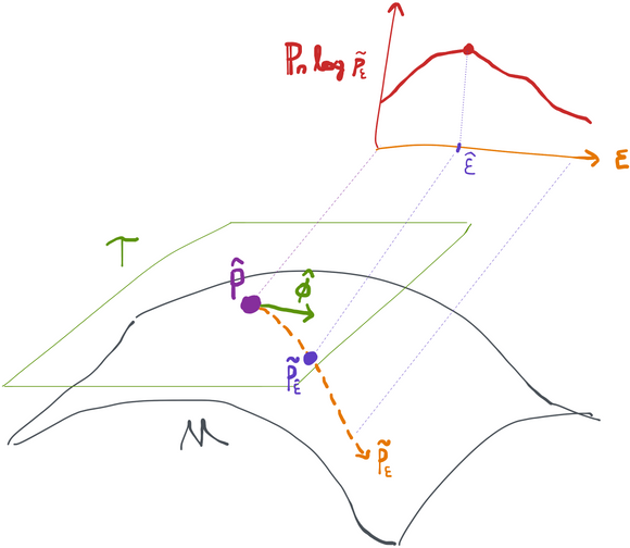
"Hardest" is defined in terms of the asymptotic variance of our best possible estimator. In other words, if we were to forget about the larger model and only consider statistical estimation within the submodel , what could we say about the minimum attainable asymptotic variance if we were trying to estimate ?
As argued below, this is a parametric model with a single parameter . For the moment, let's consider the problem of estimating the maximizer of the true log-likelihood under . In other words, we're looking for the distribution in the path that is most like . Obviously that will be itself (i.e. ). But if we didn't know that a-priori and we had to estimate using the data, what could we say about the asymptotic variance of our estimate ?
Since this is a parametric model, we can use the Cramer-Rao lower bound, which says that the minimum possible asymptotic variance that a RAL estimator of a univariate parameter can attain is . This is the inverse Fisher Information for the parameter at 0 (i.e. the true value). Using the definition of the path you can see that this is the same as (for a path that goes in some direction / has score ).
The reason this is useful is because now we can consider the plug-in . What is the asymptotic variance of this plug-in? First off, we have to realize that within the path, is a univariate function of alone. The delta method tells us that the asymptotic variance of a function of an estimated parameter is given by (i.e. evaluated at the truth) times the asymptotic variance of the estimate for the parameter. Using our fundamental identity relating the pathwise derivative and a covariance between score and gradient, we have that this term is the same as (our path starts at ).
Putting it together, our best-case scenario is that the asymptotic variance of is , or, geometrically in , . From this it is immediate (e.g. from Cauchy-Schwarz) that gives the maximum value. Since this is the best-case asymptotic variance, and higher is worse in terms of estimation, we have that the path in the direction of gives us the worst possible best-case asymptotic variance among all paths.
Intuitively, what makes certain model-parameter combinations in difficult to estimate in parametric models is that there are cases where you can change the distribution just a tiny bit, but the target parameter changes a lot. That's bad because if you try to fit the data and you get some estimated distribution, you still have a lot of uncertainty about what the parameter is: slightly different data would give you a slightly different estimated distribution, but possibly a big difference in the estimated parameter. So that is the "intuitive" meaning behind optimal asymptotic variance for a parameter in a parametric model and explains why "hardness" of the estimation problem is inherently linked to the minimum attainable asymptotic variance.
Since and are fixed (i.e. we already estimated them), the space of models that lie along this path (i.e. ) is a parametric model space with a single parameter: . As such, we can do boring old maximum likelihood estimation to find a value that maximizes the log-likelihood of along this path:
If you prefer, you can also write this out very explicitly as so you can see it's clearly a single-dimensional optimization problem in (again recall and are fixed functions by now).
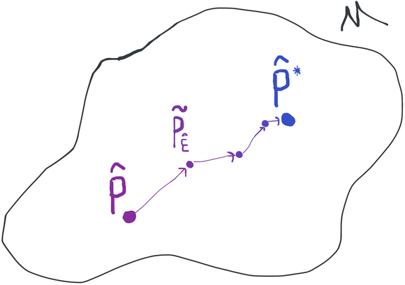
The game now is to iterate our initial guess according to the formula
at each step replacing the previous plug-in estimate and its influence function with the result of the previous iteration ( and the corresponding ). At each step we are always moving in the direction of whatever the hardest submodel is at that point and we always increase the empirical log-likelihood relative to the previous plug-in estimate. We do this until the algorithm converges, i.e. . This must occur eventually unless the empirical likelihood is unbounded over the model space, which wouldn't make any sense. At this point we declare , our final plug-in estimate of the distribution.
Something cool about this is that we've managed to take something that is generally impossible (maximum likelihood in infinite dimensions) and replaced it with a series of maximum likelihood estimation problems, each of which is one-dimensional. This is why this approach is called targeted maximum likelihood: at each step, we're solving a maximum likelihood problem, but we've targeted it in a way that helps estimate our parameter of interest.
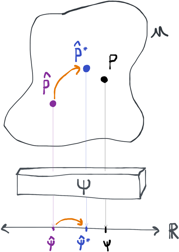
What is maximum likelihood estimation?
In case you're not familiar with it, maximum likelihood estimation is a general-purpose technique most commonly used in parametric model spaces. The goal is to find the distribution in the model that maximizes the empirical log-likelihood of the observed data. We're trying to answer the question: "of all the possible probability distributions in the model, which is the most likely to have generated the data that I observe?". Or, formally, . "Likelihood" is just a term that we use to describe the density when we're talking about it as a quantity that itself isn't fixed (in the sense that we don't know what the true density is so we have to consider multiple options). If are assumed independent and identically distributed, the density factors over and if we take a log (the argmax is the same either way) the product becomes a sum so we get . We can also use the more condensed notation .
This strategy is most often only usable for parametric models. If we have a parametric model, the maximum likelihood problem can be equivalently stated as . The advantage of this is that we've reduced the problem of looking at every possible distribution in to a problem of looking at all possible values of the parameter , which is a finite-dimensional vector space like . If the log-likelihood function is differentiable in , this is a classical optimization problem, the kind of which is solvable using tools from calculus. In particular, if as a function of is maximized at some value , then we know that the derivative at must be 0. For simple models (e.g. linear regression) there is often an analytical solution which gives , but generally you can use algorithms like gradient descent to find the maximum (or minimum if you put in a minus sign). The quantity is called the score with respect to and exactly corresponds to a path in the model space where we increment by some small amount. You can think of it as the sensitivity of the log-likelihood to small changes in the parameters (which is different at each point ). When has multiple components, the score is a vector of partial derivatives , each of which may be called the score of . We call a set of score equations (the free variable here is ) and we say that the maximum likelihood estimator solves these score equations because at we know we have to have .
All of this falls apart very quickly if you work in nonparametric model spaces because we can't transform the maximum likelihood problem into a finite-dimensional optimization. How do you search over an infinite dimensional space? Even if you have a sensible way of writing the densities in your model as a function of an infinite dimensional parameter, (e.g. another function, say say ), then for each "index" you have a score , which means you need to solve an infinite number of score equations.
However, it remains to show that this actually gets us anywhere useful. In particular, we haven't explained why we're always moving in the direction of the hardest submodel. Why not pick some other direction (score) ? We'd still be increasing the likelihood at each step, after all.
Well, here's the answer. Remember that at each step, is the maximizer of , which is a univariate function of . We know from calculus that the derivative of the maximized function at the maximizing value must be zero: . Moreover recall that for a path in a direction , we have that . After a certain number of iterations, we know that our algorithm converges, so , (and the direction is ). Putting that all together we get
This is precisely the plug-in bias term for the plug-in estimator , and we've shown that it is exactly 0. That explains why we need to move in the direction of the gradient at each iteration in the targeting step. If we were to move in a different direction we wouldn't end up cancelling the plug-in bias at the very end.
There is also an intuitive reason for choosing to move in the direction of the gradient, which is (as we've called it) the hardest submodel. This model is the hardest to estimate in because small changes in the distribution can create large changes in the target parameter. So by perturbing our estimate in the direction of the hardest submodel, what we're doing is finding the smallest possible change to our initially estimated distribution that creates the biggest possible debiasing effect in the parameter estimate.
Submodels that Span the Gradient
It's easiest to come to terms with TMLE if you think in terms of one-dimensional submodels where the path is always in the direction of the canonical gradient. However, the algorithm actually works the same if instead of one-dimensional submodels, you pick -dimensional submodels that still spans the canonical gradient at each step. What I mean by this is that often you can decompose the canonical gradient into separate pieces (we saw an example of this in the previous chapter). Then, instead of creating a one-dimensional submodel in the direction , we can create a two-dimensional submodel where .
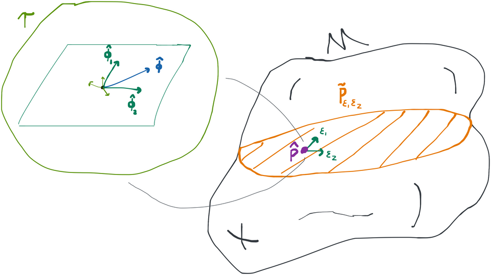
We say this submodel spans the gradient because the 1-dimensional path we were using before is actually included in this model if we let . It turns out that's all we need: the targeting step works equally well as long as the canonical gradient can be made up out of a sum of the scores for each parameter . In the targeting step we now need to replace optimization over with optimization over , but this can in fact be easier than optimization over a single because of the way the distribution factors. If the different directions in the submodel correspond to scores that are orthogonal, and each of these scores corresponds to an independent factor of the distribution, then we can perform the search for each independently from the others (i.e. temporarily setting for ). You should try to rigorously verify for yourself why that is true (and/or draw a picture!).
At any rate, we still end up with at the end of the targeting step if we work with these larger submodels. You can again verify that is the case for yourself by following the outline we used above for the one-dimensional case.
Different Paths with the Same Score
Up until now we've only been working with paths (or submodels) that look like . However, it's possible to build paths that are defined differently but which still have the same score. This is because the score just needs to determine the initial "direction" of the path- after that it can do whatever it wants. As far as TMLE is concerned (or actually the definition of regularity, etc., for that matter) a path can actually be any function of , , and such that (i.e. this path has score ) and (the path starts at ). Our paths up until this point, e.g. are just one possible example. An alternative example is with some normalizing constant to make sure that the result integrates to 1. It's actually really nice that we have so much flexibility in choosing the path because different formulations may be much easier to work with in terms of finding at each step.
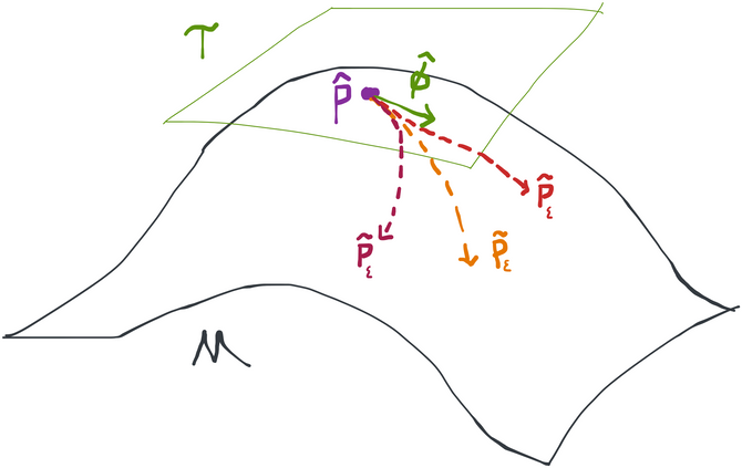
Three different paths that all start at and have score .
Therefore, no matter the definition of the path, as long as:
(i.e. it starts at our current estimate and has score equal to its canonical gradient), then this path will be valid for the targeting step.
Given this understanding, you should also now realize that there isn't one single hardest submodel. It's only after we decide on a fixed functional form of the submodel in , , and that a hardest submodel becomes uniquely defined by setting .
Locally and Universally Least-Favorable
Since we have freedom in choosing whatever form of path is most convenient for us, you might wonder if there is some automated way in which the estimation problem might be able to dictate what path is most convenient. This leads to the idea of a universally least-favorable submodel (or universally hardest path, etc.).
Up until now, the only constraints we've put on our paths have been local constraints in the sense that we only care about how the path behaves at its very beginning: it has to start at and it has to start out in the direction of . After that we don't actually care what the path does. That means that if we want to pick among these many possible paths, we have to decide on what we want the path to look like in a universal sense (i.e. at all points along the path, not just at the beginning).
Well, why not just extend our local score condition to the rest of the path? We already have that at we want , which we can write in a different way as . So why impose that condition universally instead of just locally? That would give us . Any path starting at that satisfies this condition is what we call the universally least-favorable submodel.
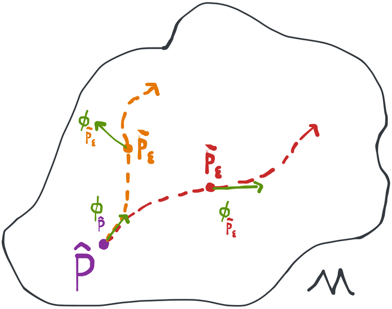
These two paths are both locally least-favorable, but only the red (rightmost) path is universally least-favorable.
This path is universally least-favorable because it goes in the hardest direction at each point . To be clear, though, what that direction is can and most often does change as we traverse the path. So it's not that the path is a "straight line" that keeps following the original gradient no matter what. Instead, this is a path that reevaluates what the hardest direction is after each infinitesimal step and then course corrects to follow it at all times.
For a given estimation problem it might take a little math to be able to express what the universally least-favorable path actually is. But once we have it our lives do get easier in one sense: if we do an iteration of the targeting step along the universally least-favorable path we get to the final targeted estimate after just one step! Why? Because the universally least-favorable path that starts at the update coincides with the continuation of the universally least-favorable path from . So if was the maximizer of the log-likelihood along the latter path, it's still the maximizer along the path that starts from there because the two paths coincide. Thus subsequent updates will not change the distribution and this proves that the targeting step converges after just one iteration. For this reason, a TMLE that uses a universally least-favorable submodel is sometimes called a one-step TMLE.
Example: ATE in Observational Study with Binary Outcome
If this all sounds terribly abstract to you, don't worry, you're not alone. Let's work through our familiar example and see where it gets us.
As in our demonstration of the bias-corrected plug-in estimator, presume we've gotten an initial estimate by modeling , , and the marginal density of with the observed empirical distribution . That's the full distribution.
As before, we know the efficient influence function for at is given by
Defining a Valid Submodel
We need to construct a submodel through that spans the score . How do we do this? Well, we can start brute-force computing stuff, or we can recall that the efficient influence function equals a sum of orthogonal scores in the tangent spaces , , and because the distribution is a product of independent factors. Specifically, we have:
Now in each iteration we can update the densities , , and separately because each of these scores can only affect its respective density. So although we're really trying to optimize in a three-dimensional submodel with parameters , the solution in this particular problem is the same as if we did the optimization separately for each of , , and . This is what I meant when I said earlier that operating in a higher-dimensional submodel could actually make things easier.
Submodel for
Let's start with the marginal distribution of , which according to our initial estimate is . The empirical log-likelihood of the data points is actually already maximized at the empirical distribution (which is why it's sometimes called a nonparametric maximum likelihood estimate). That means that no matter where we are in (or even which direction we build a path along) the optimal perturbation will always be because we're already at a maximum. Thus the targeting step will never update this part of the distribution so we already have our plug-in for the marginal distribution of the covariates: .
Submodel for
For the distribution of , we see that no matter how we define the path at each point , the fluctuation will always be because . So that distribution will also stay the same from iteration to iteration. Thus .
Submodel for
Now, finally, we come to the distribution of . Here we need to find (I'll just refer to from here on out since the other components don't matter) to maximize .
Remember that we can construct the path any way we like as long as it starts at the initial estimate and the derivative of the log-likelihood of at is the efficient influence function . Therefore I propose using this path:
Obviously if we have so this path starts at . It remains to prove that it has the right score, i.e. . I show this in the toggle below if you're curious- it just takes some algebra and derivatives.
Proof that
Abbreviate so that our definition of the path is . Taking a derivative w.r.t. on both sides and applying the chain rule gives , or, equivalently, . Again by the chain rule we know . Combining these two facts gives .
Our likelihood is if and if , so a little algebra shows that can be equivalently written as . Combining this with the above gives the desired result.
Targeting
Ok, we've got our path, so how do we find ? This is where things clean up nicely. The way we constructed our submodel, is just the coefficient we get if we regress the vector of onto the "clever covariate" vector of with a fixed offset using logistic regression!
Proof that this is logistic regression with a fixed offset
We can write the conditional likelihood for a binary variable where like . This shows that the log-likelihood is
Moreover we have from our construction of the path that . Plugging in and the definition of (tilde or hat) immediately gives that
Compare this to the definition of logistic regression (e.g. eqs. 12.7 and 12.4 here). I've included underbraced quantities to the above so you can directly map the notation.
The only difference with the usual logistic regression is that in our case, we have a fixed intercept and a fixed coefficient . This is known as an "offset" in the literature about logistic regression and options to use offsets exist in practically every software package that implements logistic regression. The coefficient is what we fit using the "data" , which is precisely the solution to , as desired.
After fitting our logistic regression and extracting the coefficient , the final thing we have left to do is to update the distribution. For this we just have to compute , which in terms of means
This is now a fixed function that we can evaluate at any value of .
Iterating
We can now repeat what we did above, at each step plugging in the result from the previous iteration into the role played by the current estimate . However, the way we've worked out the submodel in this case implies that after the first iteration. Intuitively, that's because we already regressed onto in the first iteration, so subsequent regressions don't change anything. You can formally prove this to yourself if you like, but it's not actually that important. This suggests that the path we chose is universally least-favorable.
Since we've converged already, our final estimate is exactly the function shown in the display above. We can now execute the plug-in and that's our final estimate.
Efficiency
We've now explained the TMLE algorithm and how it guarantees that the plug-in bias for the targeted plug-in is 0. Of course, since TMLE is a plug-in, we can analyze its efficiency using the exact same expansion as we did for the naive plug-in:
It remains to show that the empirical process term and second-order remainder are both still even though we've replaced our initial plug-in (for which we know these terms are as long as we do things sensibly) with the targeted plug-in . In other words, we need to make sure that by eliminating the plug-in bias via targeting we haven't messed up the good things we already had going for us.
Thankfully, it turns out that we're still in business. The heuristic argument for why is that at each iteration of the targeting step, we're always increasing the empirical log-likelihood of our plug-in estimate. Since each update is done with a parametric model, we're also guaranteed that this contributes only an error of order relative to increasing the true log-likelihood . Thus we can claim that the true log-likelihood of our estimated distribution is always increasing (to a first-order approximation). That, in turn, implies that the KL divergence between and decreases at least at the same rate (in ) that the original plug-in attains. This implies that also attains that rate (in norm). Finally, using something called the functional delta method, we can infer that nuisance parameters (which are functionals of the density) also maintain their rates of convergence. You'll recall from the section on the naive plug-in that these are the quantities that we need to converge in order to eliminate the empirical process and 2nd order remainder terms. As a result of all of this, we can say that any conditions required to satisfy the rate for these terms indeed are maintained through the targeting step, and thus TMLE produces an efficient estimator.
Discussion
Deriving and implementing a TMLE for a given estimation problem generally takes more work than doing a bias-corrected or estimating equations estimator. Since all three give asymptotically equivalent results, why should we bother?
Well, as we've already noted, bias-correction and estimating equations each have their own problems. Sometimes they "blow up" or produce estimates that are outside of the natural range of the parameter. Sometimes you can't even construct the estimating equations estimator and sometimes the bias-corrected estimator isn't able to take advantage of the double robustness of the estimation problem.
TMLE, on the other hand, has none of these problems. What makes TMLE so robust is that it goes back to the original plug-in philosophy: all we're doing is estimating a distribution for the data and then asking what the value of the target parameter is for that distribution. There's no fudging based on a bias correction or trying to brute-force solve an estimating equation (though the final TMLE plug-in does satisfy the estimating equation). Since it's a plug-in, the TMLE can't help but respect any bounds on the parameter. That also typically makes it harder to blow it up. In general, you can expect estimators built with TMLE to behave more reasonably and consistently in finite samples.
"Blowing up" an estimator
We saw that the bias-corrected and estimating equations approaches give the same estimator for the ATE problem, which we called AIPW. The form of this estimator is a sample average over terms where one of the factors is . If the estimated propensity score is close to 0 or 1 for some subjects in the study, that factor ends up being massive and it completely dominates the sample average. Of course, in an infinite sample, that couldn't happen because some other subject would have an equally large weight in the other direction or the large weight would be balanced with many subjects with smaller weights. But we don't have infinite data. We have finite data. That makes the AIPW estimator unstable in finite samples where there are strong predictors of treatment assignment. The only way to address this is to use ad-hoc methods like weight stabilization or trimming.
On the other hand, the TMLE estimator doesn't incorporate terms of the form directly into a sample average. Instead, it uses them as a covariate in a linear adjustment of the original regression model . That makes the procedure more stable in the face of small or large propensity scores. This comes automatically. There are also additional variations on TMLE (e.g. collaborative TMLE) that are theoretically justified and which do even more to improve the finite-sample robustness of the resulting estimator.
Besides the practical benefits, TMLE has a lot going for it in theory. As I touched on earlier, TMLE is the "natural" extension of maximum likelihood estimation to cases where it is impossible to carry out the explicit optimization problem in infinite dimensions. TMLE beautifully reduces this problem to a series of lower-dimensional maximum likelihood problems by correctly identifying the right direction to move in within the statistical model.
Moreover TMLE leaves a lot of room for well-motivated variations. Different choices of submodels or additional scores (remember the submodel just has to span the gradient, but it can include additional directions if desired) can give TMLE more beneficial properties. There is also collaborative TMLE, in which components of the distribution that don't get updated by the targeting step (e.g. in our ATE example) are fit in such a way that they maximize the benefit of targeting instead of just to minimize a generic loss function. Finally, TMLE admits natural extensions to attain higher-order efficiency (i.e. cancelling second-order bias terms), which is challenging in the bias-correcting and estimating equations frameworks.
In short, TMLE has all of the advantages of historical approaches in the sense that it can leverage flexible machine learning models and effectively minimize or any eliminate statistical assumptions. However, it eliminates most of the drawbacks of those methods and even leaves room for further innovation.